Disaggregated LLM Serving: From PD Disaggregation to Attention Offloading

Over the past two years, the core tension in LLM Serving has become increasingly clear: as models grow larger and context windows get longer, it is no longer enough to simply “put more requests into the same batch.” The real challenge is that different phases and modules stress hardware in very different ways. Prefill wants compute. Decode wants memory bandwidth. In MoE models, Attention and Expert modules introduce yet another mismatch.

Disaggregated LLM Serving is essentially about separating components with different resource needs so that they can scale independently across GPU pools, parallelism strategies, and sometimes even storage tiers. This post follows the evolution from Continuous Batching and Chunked Prefill to DistServe, Mooncake, MegaScale-Infer, and Adrenaline.

1. Starting From Autoregressive Generation

LLM inference usually has two phases:

1. Prefill: processes all prompt tokens at once and produces the first output token. Since prompt tokens can be processed in parallel, Prefill is usually compute-bound and mainly affects TTFT (Time To First Token).
2. Decoding: generates subsequent tokens one by one. Each step reads the historical KV Cache, so Decoding is usually memory-bandwidth-bound and mainly affects TPOT (Time Per Output Token) or ITL (Inter-Token Latency).

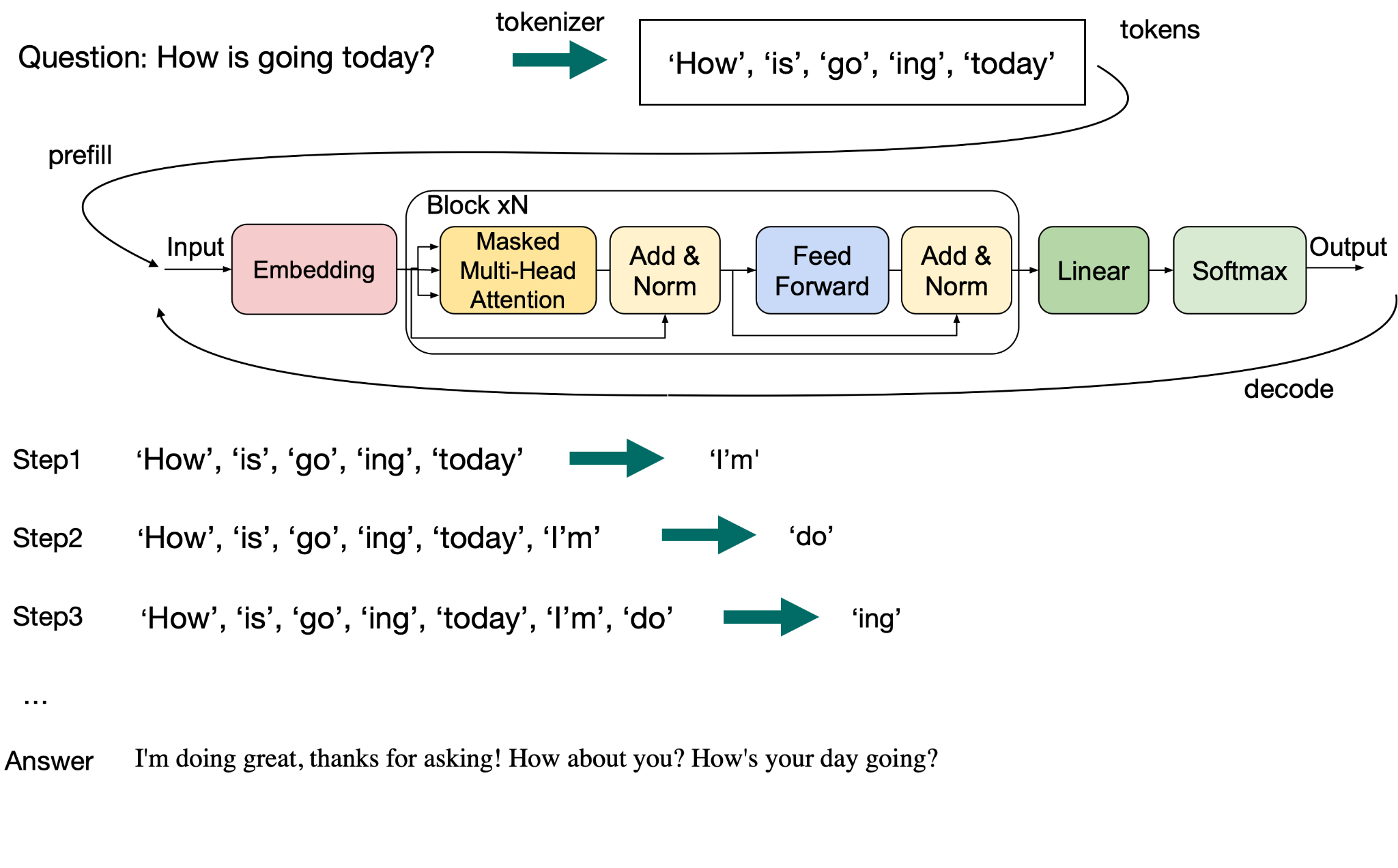
This figure is useful from two angles:

1. Token dependency: Prefill consumes the whole prompt, and prompt tokens can enter the model in parallel. Decoding can only generate one new token at each step, and each next token depends on the previous output.
2. KV Cache evolution: Prefill writes KV Cache for all input tokens. Each decoding step reads existing KV Cache and appends KV for the new token. The longer the context, the more historical state each decode step reads.
3. Metric mapping: Prefill determines how long the user waits for the first token, namely TTFT. Decoding determines whether the following stream is smooth, namely TPOT/ITL.

This difference drives nearly all later system designs: if Prefill and Decoding are forced into the same GPU configuration, the system will repeatedly trade off TTFT, TPOT, throughput, and utilization.

2. Scheduling Optimizations Inside Monolithic Serving

Before fully disaggregating the system, earlier work mainly tried to improve batching inside a colocated architecture.

2.1 Continuous Batching: Removing Request-Level Waiting

Traditional static batching is blocked by the longest request in the batch. As long as one request has not finished, the whole batch keeps occupying its slots. Orca’s Continuous Batching lowers the scheduling granularity to token iterations: after each iteration, completed requests leave immediately and new requests fill the freed slots.

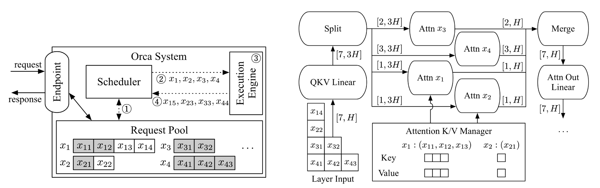
The labels 1-4 in the left half describe Orca’s scheduling loop:

1. 1. Read state from the Request Pool: the Scheduler observes the progress of all active requests. In the figure, $x_1$ already has a long history and will continue from $x_{14}$ to generate $x_{15}$; $x_2$ has generated up to $x_{22}$ and will continue to $x_{23}$. Thus $x_1,x_2$ are old requests in Decode. In contrast, $x_3,x_4$ have just entered the system and only have prompt tokens in the Request Pool, such as $x_{31},x_{32}$ and $x_{41},x_{42},x_{43}$, so they are in Prefill.
2. 2. Select requests for this iteration: the Scheduler puts $x_1,x_2,x_3,x_4$ into the same iteration. The important detail is that $x_1,x_2$ each need only one query token for Decode, while $x_3,x_4$ need multiple prompt tokens for Prefill. A single Continuous Batching iteration can therefore contain both Decode tokens and Prefill tokens.
3. 3. Execute one model iteration: the Execution Engine does not run a request to completion. It executes one model iteration. For $x_1,x_2$, this iteration generates the next token using their historical KV Cache; for $x_3,x_4$, it processes the prompt and builds their KV Cache.
4. 4. Return results: the engine returns newly generated tokens or intermediate results such as $x_{15},x_{23},x_{33},x_{44}$, and the Scheduler updates the Request Pool. If a request reaches EOS, its slot can be released immediately. Once $x_3,x_4$ finish Prefill, they will also enter the Decode queue.

The right half explains how this iteration runs inside the model. After QKV Linear, tokens from different requests are Split into separate attention tasks, such as Attn $x_1$, Attn $x_2$, Attn $x_3$, and Attn $x_4$. The Attention K/V Manager locates each request’s own historical KV Cache. After each attention task completes, the results are Merged back into a unified batch and continue through Attn Out Linear and later layers. Orca turns “request-level batching” into “iteration-level batching”: each iteration advances only one step, but each iteration can recompose the batch.

This reduces padding and idle slots, but long Prefill still shares the same iteration with ongoing Decode. Phase interference therefore remains.

2.2 Chunked Prefill: Cutting Long Prefill Into Pieces

Chunked Prefill in Sarathi-Serve further splits long prompts into chunks. Each iteration processes only one prefill chunk and combines it with Decode tokens from other requests. This smooths a large compute spike into smaller pieces and reduces decoding latency spikes.

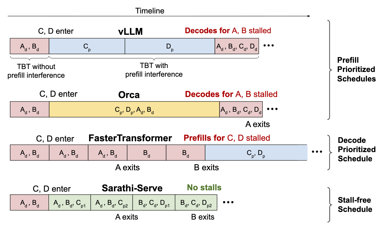
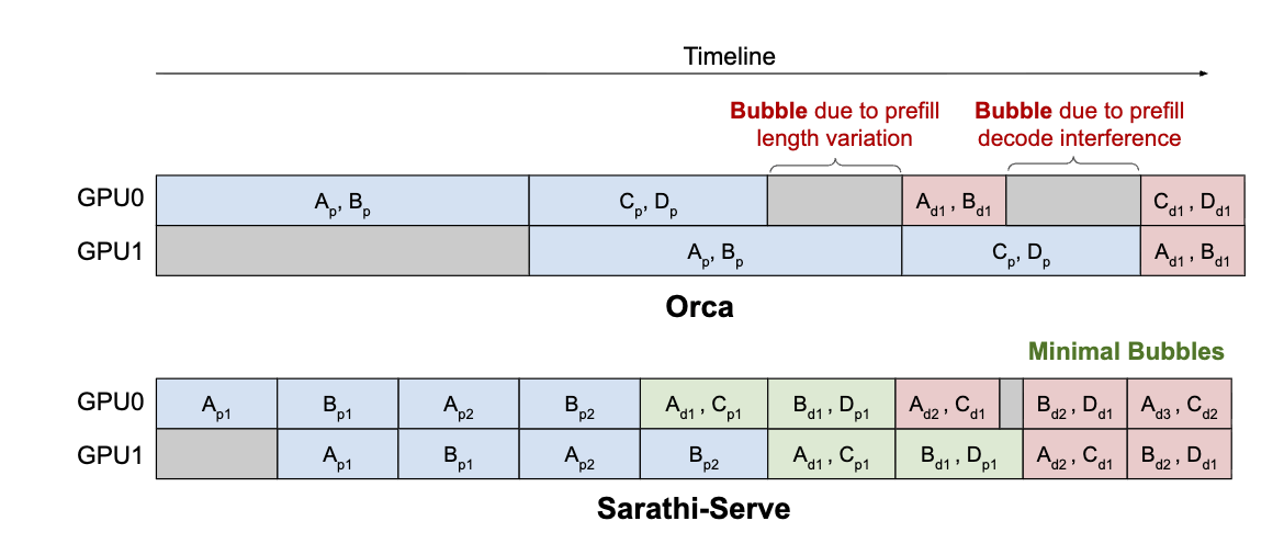
Both figures express the same idea: do not let one long prompt monopolize the GPU. Sarathi-Serve cuts a long prompt into chunks, processes only one chunk per iteration, and piggybacks that chunk with Decode tokens from other requests. This makes the workload per iteration more even, so ongoing Decode requests do not have to wait for one giant Prefill block.

The cost is also implicit in the figures: the chunked request cannot produce its first output token until all chunks finish, so its own TTFT increases. Chunked Prefill smooths latency spikes, but it is still not true resource disaggregation.

3. Why PD Disaggregation?

Prefill-Decoding Disaggregation (PD Disaggregation) is motivated by two problems: phase interference, and resource/parallelism coupling.

3.1 Phase Interference: TTFT and TPOT Hurt Each Other

In colocated serving, Prefill and Decoding are batched together on the same GPU instance. Long Prefill can block Decode tokens and increase TPOT; Decode requests also occupy batch slots and can increase Prefill queueing time and TTFT.

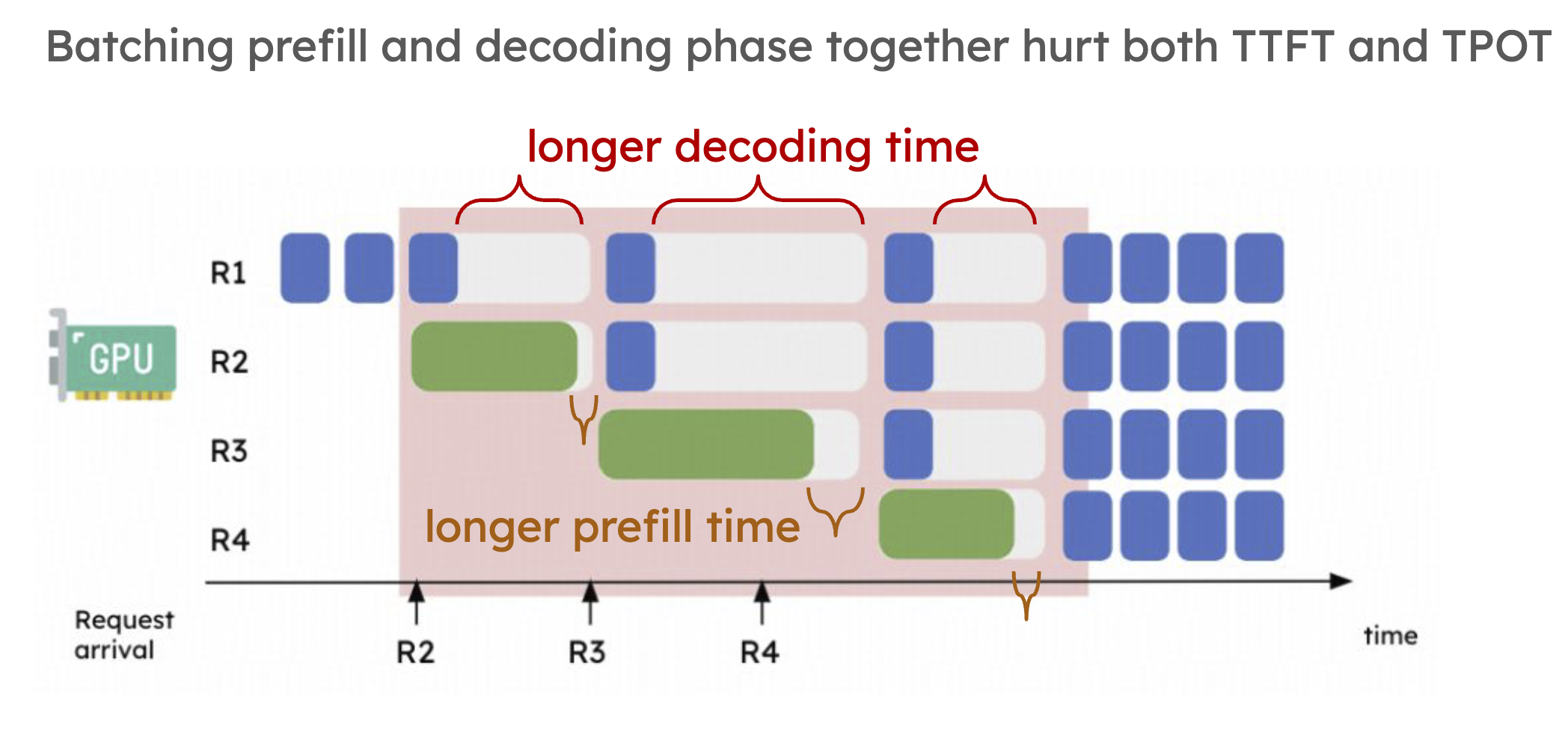
In this figure, blue blocks represent Decode tokens and long green blocks represent Prefill for new requests. Once the green block is inserted, Decode steps from other requests are stretched, which corresponds to worse TPOT. At the same time, the Prefill itself is not running alone; it is mixed with Decode workload, increasing TTFT. Mixed execution often contaminates both critical paths instead of simply filling idle resources.

Interactive chat, code completion, and summarization often specify both TTFT and TPOT SLOs. Optimizing only one of them is not enough.

3.2 Resource Coupling: One GPU Configuration Cannot Fit Both Phases

Prefill is closer to large matrix computation and often benefits from tensor parallelism to reduce TTFT. Decoding processes only one token per step and is more constrained by KV Cache reads and memory bandwidth. Large tensor parallelism also puts All-Reduce on every token’s critical path, which quickly sees diminishing returns.

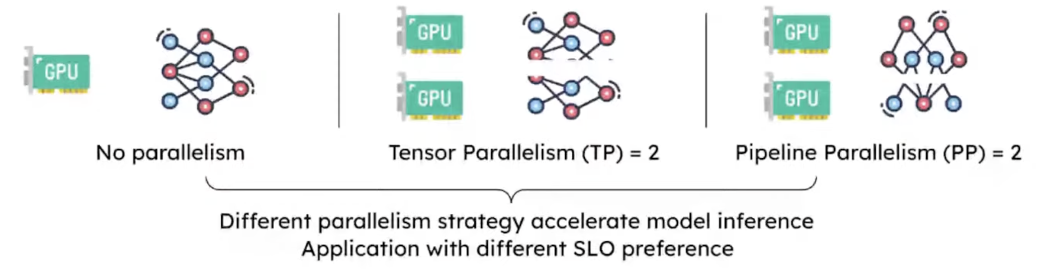
The figure contrasts parallelism strategies. No parallelism means running the full model on one GPU. Tensor Parallelism (TP) splits a layer’s matrix computation across GPUs, which helps large compute-heavy operations. Pipeline Parallelism (PP) places different layers on different GPUs, which helps scale model and KV Cache capacity. Prefill cares more about finishing a large compute block quickly; Decode cares more about per-token communication, memory capacity, and batch aggregation. Colocation forces both phases to share one TP/PP configuration.

In colocated serving, GPU allocation and parallelism must serve both Prefill and Decoding. The tighter SLO or heavier phase tends to dominate the configuration. Under some workloads, meeting Decode TPOT may require more GPUs or a different parallelism strategy, causing Prefill TTFT to fall far below its SLO and wasting resources. Conversely, if the configuration is chosen mainly for Prefill TTFT, Decode may hit TPOT SLO first due to limited batch capacity, KV Cache capacity, or memory bandwidth.

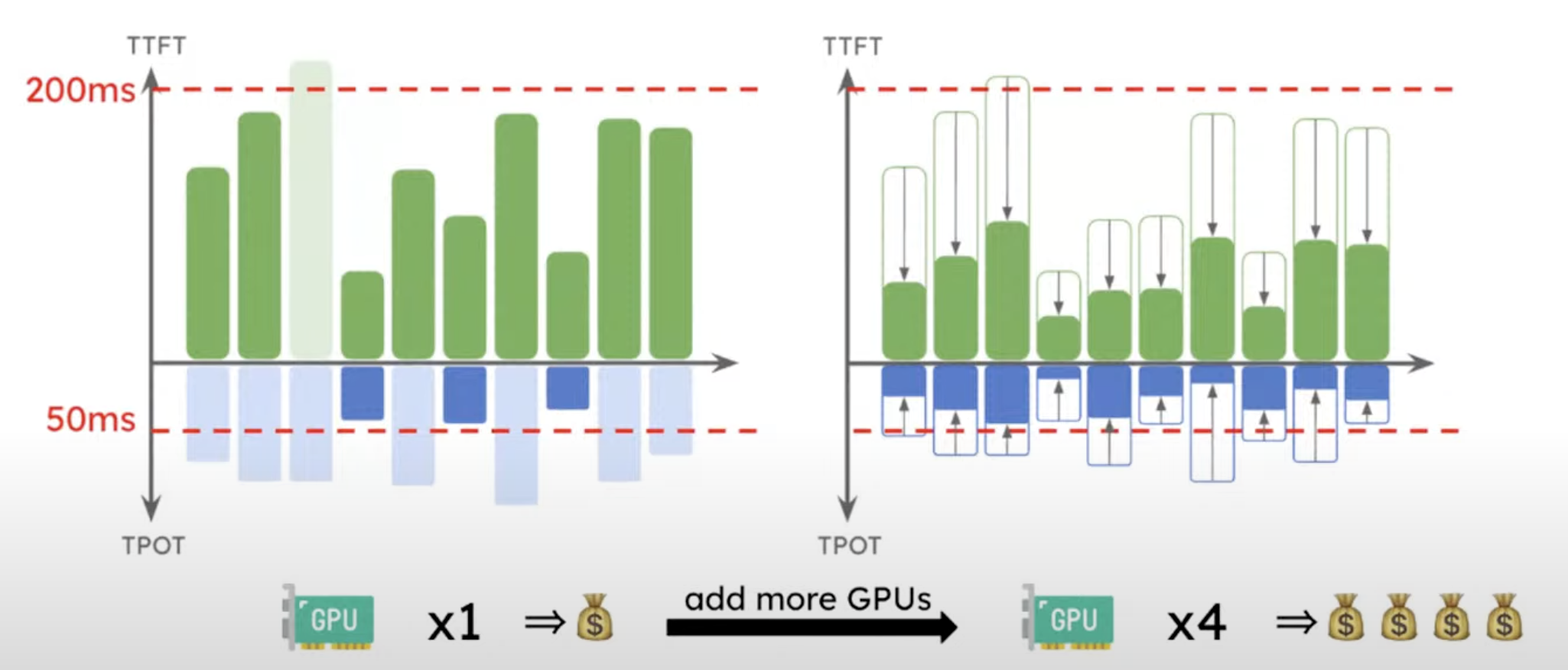
The vertical axis combines TTFT and TPOT, and the red dashed lines are SLOs. With one GPU on the left, some requests already violate TPOT. Adding GPUs on the right can bring TPOT down, but TTFT is also pushed far below its SLO. Users do not gain much from TTFT that is much faster than the SLO, but the system pays extra GPU cost for it. This is the resource and parallelism coupling highlighted by DistServe.

PD Disaggregation therefore separates Prefill and Decoding into different GPU pools so that each can choose its own resource scale and parallelism strategy.

4. DistServe: PD Disaggregation Optimized for Goodput

DistServe is a representative PD-disaggregated system. It physically separates Prefill workers and Decode workers: a request first enters the Prefill pool to process the prompt, then its KV Cache is transferred to the Decode pool for autoregressive generation.

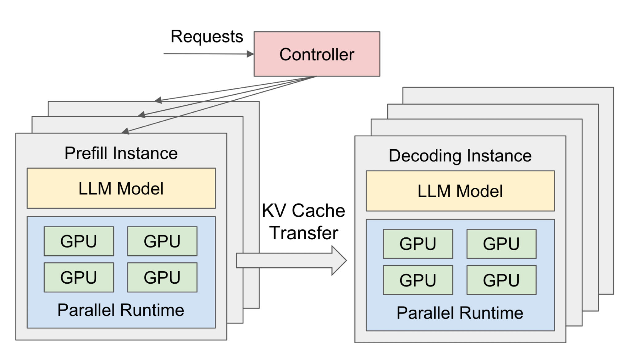
There are three key flows in the architecture. First, the Controller/Router selects a Prefill Instance first, because new requests must encode the prompt into KV Cache. Second, both Prefill Instances and Decoding Instances host the full LLM model, but their parallelism strategies and resource sizes can differ. Third, after Prefill finishes, the cross-node state being transferred is KV Cache, not the raw prompt or full intermediate activations. KV Cache Transfer is the main extra cost of PD disaggregation and the target of placement optimization.

DistServe’s key idea is not just “split the phases”, but to optimize Goodput: the maximum request rate the system can sustain while meeting both TTFT and TPOT SLOs. This is more meaningful than raw throughput for online serving, because a request that finishes after its SLO is not useful capacity.

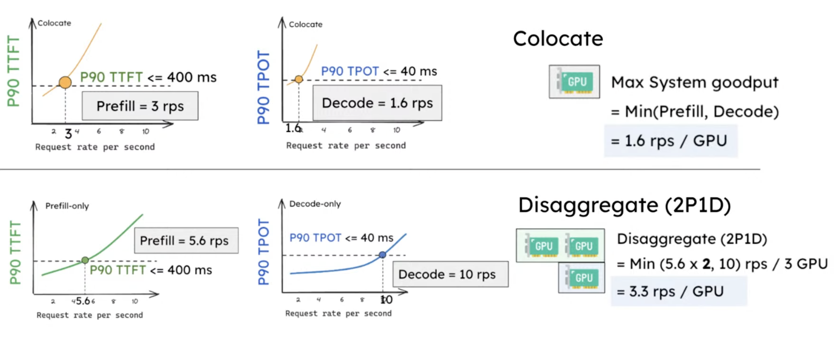
The Goodput figure should be read by looking at where each latency curve crosses the dashed SLO line. In the colocated case, Prefill and Decode are mixed, so the maximum goodput is limited by whichever phase hits its SLO first; in the figure, Decode becomes the bottleneck at about 1.6 rps/GPU. In the disaggregated case, Prefill-only and Decode-only capacity can be scaled separately. The 2P1D example makes Prefill and Decode capacities better matched and reaches about 3.3 rps/GPU. The gain is not because one phase is magically faster, but because the two SLO constraints can be satisfied independently.

After disaggregation, Prefill can use more aggressive tensor parallelism to reduce TTFT, while Decode can use a strategy better suited to KV Cache capacity and bandwidth, building a larger batch for throughput. DistServe also uses bandwidth-aware placement to keep KV Cache transfer on fast links.

The Prefill/Decode node ratio is not fixed. A better approach is to infer it from workload and SLOs: long prompts with short outputs usually stress Prefill; short prompts with long outputs usually stress Decode; tighter TTFT SLOs require stronger Prefill compute; tighter TPOT SLOs require more Decode KV Cache capacity, memory bandwidth, and batch capacity. DistServe enumerates GPU counts and parallelism strategies for Prefill and Decode, estimates their TTFT/TPOT curves, and chooses the combination with the highest per-GPU goodput. The 2P1D ratio in the figure is not universal; it is simply a good match for that workload and SLO.

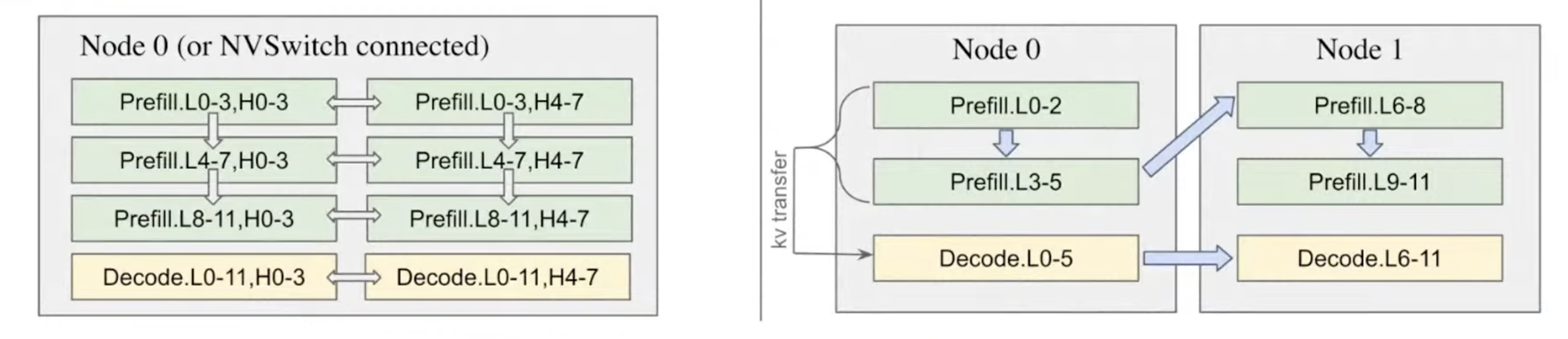
This figure shows why PD disaggregation cannot look only at GPU counts; topology matters too. On the left, Prefill and Decode are placed within the same node or NVSwitch domain so that KV Cache transfer can use NVLink/NVSwitch. On the right, when cross-node placement is unavoidable, DistServe uses bandwidth-aware placement to reduce KV Cache transfer over low-bandwidth links. Placement determines whether the communication cost of disaggregation is smaller than its scheduling benefit.

The paper reports that under strict latency constraints, DistServe can serve up to 7.4x more requests or satisfy 12.6x tighter SLOs while keeping more than 90% of requests within latency constraints.

The cost is also clear: KV Cache must be transferred across workers. If network bandwidth is insufficient, transfer latency can offset the gain. It can also introduce new utilization imbalance, such as idle memory on Prefill nodes and idle compute on Decode nodes.

5. Mooncake: Making KVCache the Center of the System

Long-context workloads push PD disaggregation further: the bottleneck is not only where computation runs, but also where KV Cache lives, how it is reused, and how it is moved.

Mooncake, the KVCache-centric serving architecture behind Kimi, separates Prefill and Decoding while also pooling underused CPU, DRAM, SSD, and NIC/RDMA resources into a distributed KVCache pool.

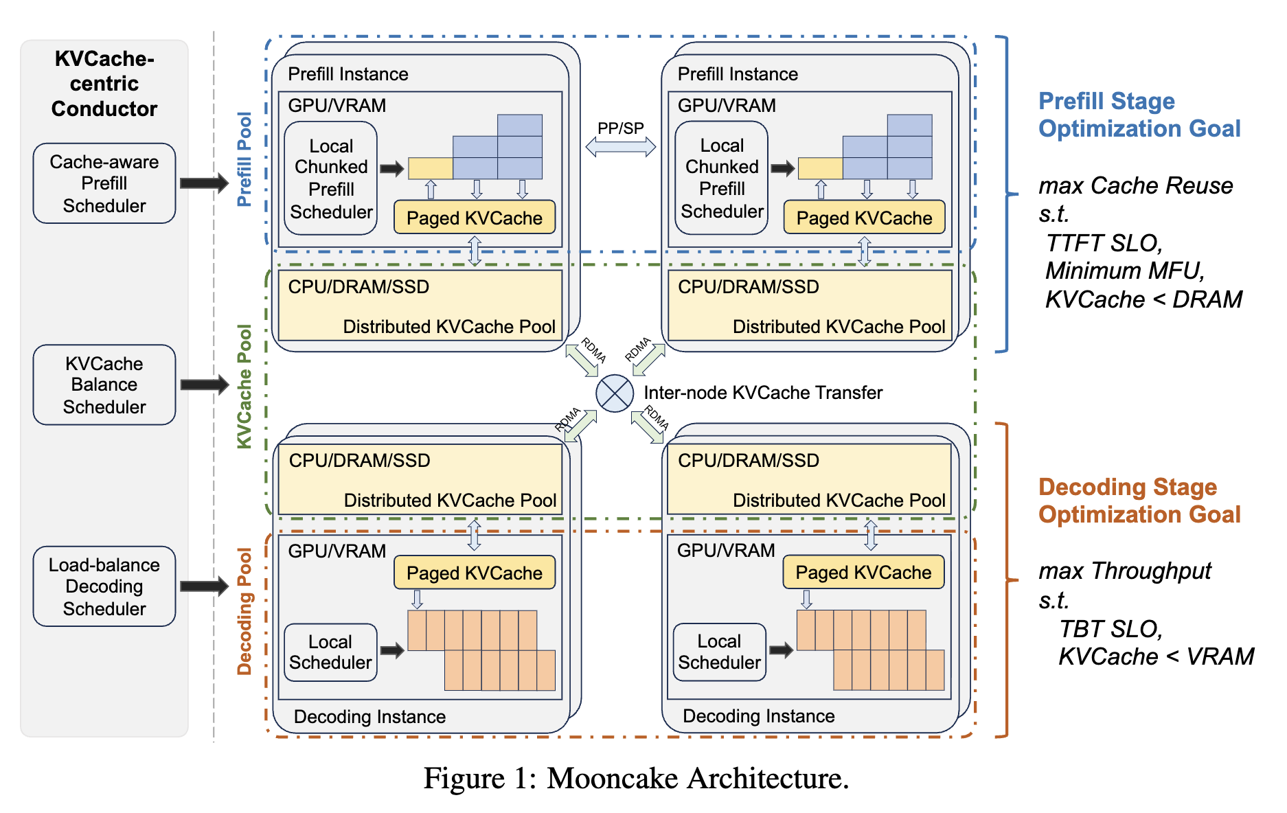
The architecture has three layers. On the left, the Conductor contains a cache-aware prefill scheduler, a KVCache balance scheduler, and a load-balance decoding scheduler, meaning it is not doing simple round-robin dispatch. In the middle, the green dashed area is the distributed KVCache Pool, which incorporates CPU/DRAM/SSD instead of relying only on GPU VRAM. On the right, the objectives are explicit: Prefill maximizes cache reuse while meeting TTFT SLO, and Decode maximizes throughput while meeting TBT/TPOT SLO.

Mooncake’s core scheduler is the Conductor. It maintains a global KVCache view and routes requests by considering cache hits, Prefill queues, Decode load, and transfer cost.

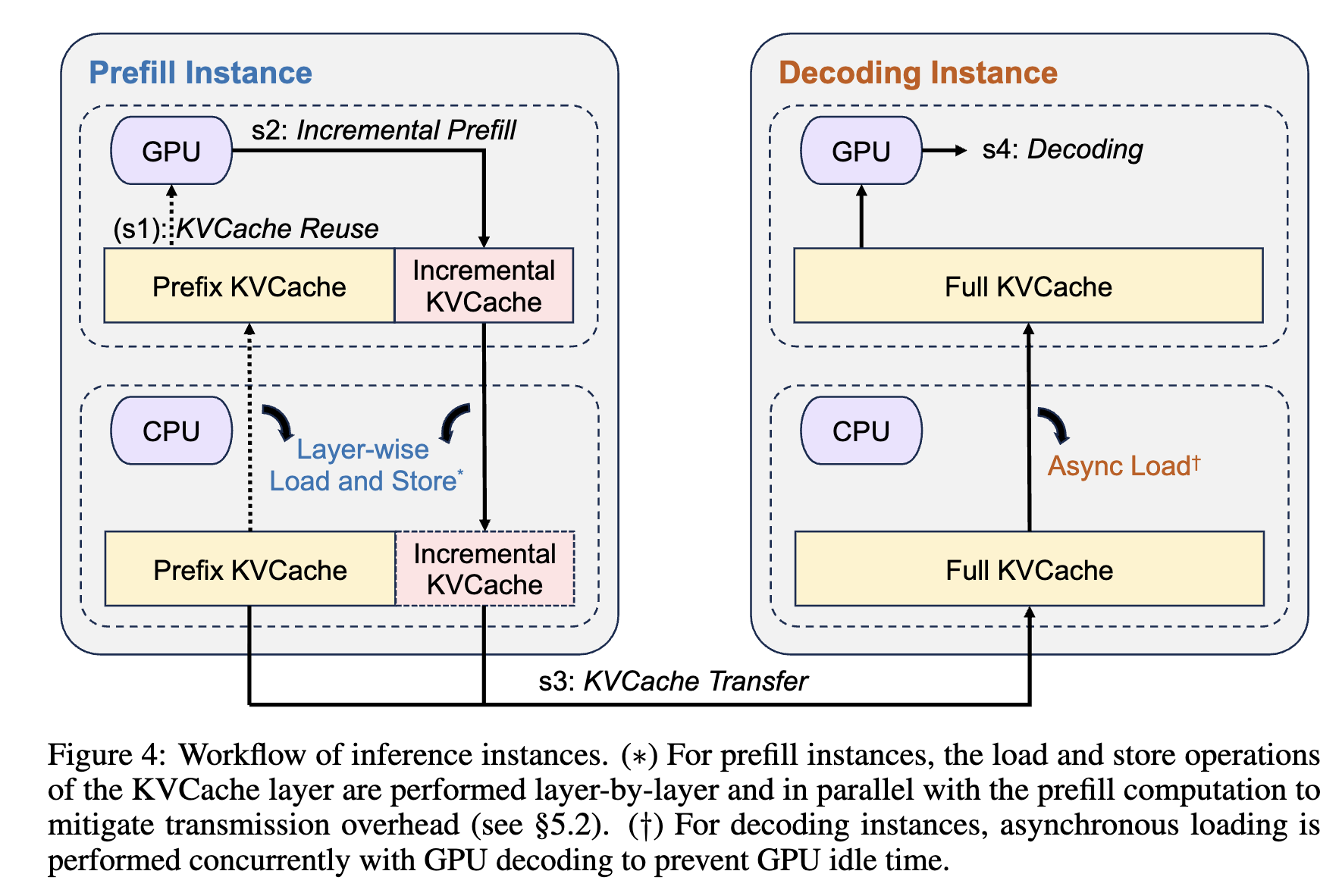
The workflow breaks one request into four steps. s1 is Prefix KVCache Reuse: if the historical context is cached, the Prefill instance reuses prefix cache. s2 is Incremental Prefill: only the new tokens are prefilling, while layer-wise load/store between GPU and CPU tries to hide KVCache movement behind computation. s3 is KVCache Transfer: complete or incremental KVCache is moved to the Decode instance. s4 is Decoding: the Decode side asynchronously loads full KVCache while generating tokens, avoiding GPU idle time.

Mooncake is especially useful for long-context workloads. The paper reports 59% to 498% higher effective request capacity on real traces, with production deployment across thousands of nodes and over 100 billion tokens per day. Its complexity is also higher: tiered-storage latency, KVCache migration, hot-spot replication, and overload protection must all be handled by the global scheduler.

6. MegaScale-Infer: From Phase Disaggregation to Module Disaggregation

PD disaggregation addresses the difference between Prefill and Decoding. With MoE models, however, a new mismatch appears inside the Decoding phase itself: Attention and FFN/Expert modules have different bottlenecks.

6.1 Motivation: Utilization Mismatch in MoE Decoding

MegaScale-Infer starts from a counter-intuitive observation: MoE reduces the number of activated parameters and FLOPs per token, but this does not necessarily reduce serving cost. GPU efficiency depends not only on total FLOPs, but also on whether those FLOPs form a large enough batch and efficient matrix multiplications.

During decoding, Attention must read each request’s own historical KV Cache. Different requests’ KV Cache cannot be shared like model weights, so Attention tends to be memory-bound and sees low GPU utilization. FFN is different: it mainly reads model weights, and the same FFN weights can be reused by all tokens in the batch. As batch size grows, FFN GEMM becomes larger and can better saturate GPU compute.

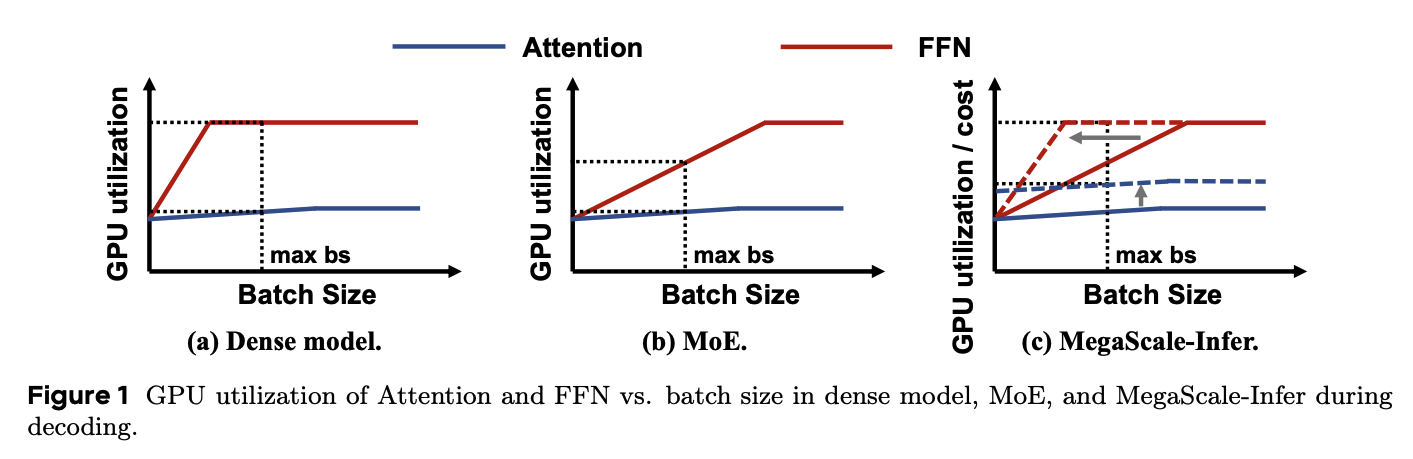
The three subfigures correspond to a dense model, a regular MoE model, and MegaScale-Infer. The blue curve is Attention and the red curve is FFN. In a dense model, each layer has one FFN and all tokens go through it; within the maximum batch size allowed by memory and latency constraints, the FFN usually forms a large enough GEMM and quickly reaches high utilization.

MoE changes this. We need to distinguish global batch size from effective batch size per Expert. The former is the number of requests processed in one decode iteration; the latter is the number of tokens actually routed to one Expert by the Gate. Since each token selects only top-k Experts while the total number of Experts is often large, each Expert sees only a fraction of the global batch. In large MoE configurations, that fraction may be less than one quarter or even an order of magnitude smaller. The resulting GEMM becomes small, so MoE FFN can degrade from compute-intensive to memory-intensive, producing the slow-rising red curve in regular MoE.

MegaScale-Infer separates Attention and Expert modules so they can scale independently. Attention modules are replicated with data parallelism, while Expert modules form an expert parallel group and receive tokens from multiple Attention replicas. The key effect is consolidating requests from multiple Attention replicas on the Expert side: each Expert sees more tokens, making FFN more likely to return to the compute-intensive, high-utilization regime. This is what the dashed curve represents.

The point is not that “MoE is slow”; rather, Attention and FFN need different scaling strategies. If they are tied to the same GPU pool, it is hard to keep Attention access, Expert weight access, and communication cost all in an efficient region.

6.2 Background: MoE Layer and Expert Parallelism

In an MoE layer, Attention is dense and all tokens participate in it. FFN becomes sparse Experts, and each token is routed by the Gate to only a subset of Experts. Traditional Expert Parallelism places different Experts on different GPUs or nodes and exchanges tokens through All-to-All communication.

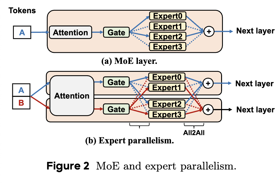
The top half shows a single MoE layer: tokens go through Attention, then the Gate selects Experts, and Expert outputs are aggregated before the next layer. The bottom half shows Expert Parallelism: different Experts are placed on different devices, so tokens A and B may be routed to different Experts. All-to-All sends tokens to selected Experts and then sends results back. This communication is fundamental to MoE scaling, but it can amplify scheduling and communication cost when batches are small or routing is sparse.

Expert Parallelism follows MoE’s sparse routing structure: different Experts live on different devices, tokens are sent to the selected Experts, and results are gathered back. Its problem also comes from the same sparsity: each Expert sees only part of the global batch. When too few tokens land on one Expert, FFN cannot form a large enough GEMM and GPU utilization drops.

6.3 AE Disaggregation: Scaling Attention Nodes and Expert Nodes Separately

MegaScale-Infer further separates Attention and FFN/Expert inside the Decoding phase, forming Attention-Expert Disaggregation (AE Disaggregation). Attention nodes store Attention parameters and KV Cache and can be replicated with data parallelism. Expert nodes store Expert parameters and form an expert parallel group. Tokens from multiple Attention replicas can be consolidated on Expert nodes, increasing each Expert’s effective batch size.

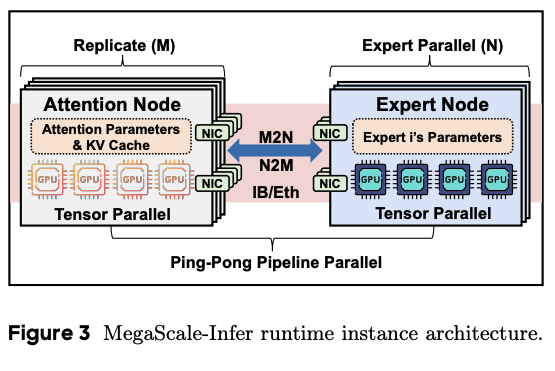
In the runtime architecture, the left side has M Attention Node replicas, each storing Attention parameters and KV Cache and using Tensor Parallelism within the node. The right side has N-way Expert Parallelism, with each Expert Node storing part of the Expert parameters. The M2N/N2M communication in the middle means token hidden states flow between Attention and Expert sides. The bottom Ping-Pong Pipeline Parallel label indicates that the system streams micro-batches instead of waiting for a whole batch to finish before transfer.

This split brings three benefits:

1. Independent scaling: Attention and Expert can use different GPU counts according to their bottlenecks.
2. Heterogeneous deployment: Attention can use nodes better suited for KV Cache and dense attention access, while Expert can use nodes better suited for large weight storage and FFN compute.
3. Larger effective Expert batch: tokens from multiple Attention replicas are consolidated on the Expert side, making Expert computation more compute-bound.

The Attention/Expert node ratio is also not fixed. Attention is constrained mainly by KV Cache capacity, memory bandwidth, and decode latency. Expert is constrained mainly by effective batch size per Expert, FFN compute time, and routing balance. Too few Attention replicas make KV Cache access or Attention compute the bottleneck. Too few Expert nodes queue FFN compute. Too many Expert nodes reduce tokens per Expert, shrink GEMMs, and lower utilization. MegaScale-Infer therefore uses a performance model to search deployment plans where Attention micro-batch time and Expert micro-batch time are close, while A2E/E2A communication can be hidden by computation.

To reduce communication overhead, MegaScale-Infer uses a customized M2N communication library that removes unnecessary GPU-to-CPU copies, communication group initialization overhead, and global GPU synchronization.

6.4 Ping-Pong Pipeline: Hiding Communication With Micro-Batches

AE disaggregation introduces a clear cost: tokens must frequently move between Attention nodes and Expert nodes. MegaScale-Infer therefore introduces Ping-Pong Pipeline Parallelism. The four lanes are Attention, A2E transfer, Expert, and E2A transfer; the horizontal axis is time; each block represents a micro-batch at a layer.

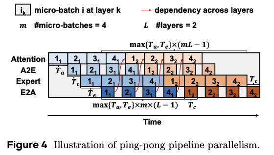
Here $m=4$ means the batch is split into 4 micro-batches, and $L=2$ means the example shows 2 layers. Each $i_k$ block means the $i$-th micro-batch at layer $k$. The red diagonal lines mark cross-layer dependencies: the same micro-batch must receive its E2A result from the previous layer before entering Attention in the next layer. $T_a$, $T_e$, and $T_c$ roughly represent Attention compute time, Expert compute time, and communication time. The total time depends on $\max(T_a, T_e)$ and $T_c$, meaning a full pipeline tries to use the slower compute stage to cover the other compute stage and communication.

The goal is to cover A2E/E2A communication with Attention or Expert compute. The paper reports up to 1.90x higher per-GPU throughput than state-of-the-art MoE serving systems. However, this design is sensitive to network latency and jitter; if M2N/N2M communication cannot keep up, pipeline bubbles directly reduce throughput.

7. Adrenaline: Offloading Decode Attention to Prefill

After PD disaggregation, a new utilization problem appears: Prefill nodes are compute-busy but may have idle memory capacity and bandwidth, while Decode nodes are memory/bandwidth-bound but often have idle compute. Adrenaline exploits this complementarity.

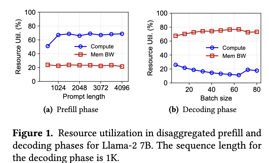
This figure is the motivation for Adrenaline. In the Prefill phase on the left, compute utilization remains high as prompt length increases, but memory bandwidth utilization is low, indicating spare memory capacity and bandwidth on Prefill instances. In the Decoding phase on the right, memory bandwidth utilization is high while compute utilization is low, indicating that Decode instances are bottlenecked by KV Cache access. Adrenaline uses this complementarity by moving memory-bandwidth-heavy Decode Attention to the Prefill/Attention Executor side.

Adrenaline’s core idea is to offload part of the Decoding phase’s Attention computation, the part that heavily reads KV Cache, to Prefill nodes. Decode nodes keep lighter Q projection and FFN work, send Query to Prefill nodes, and receive the Attention output back.

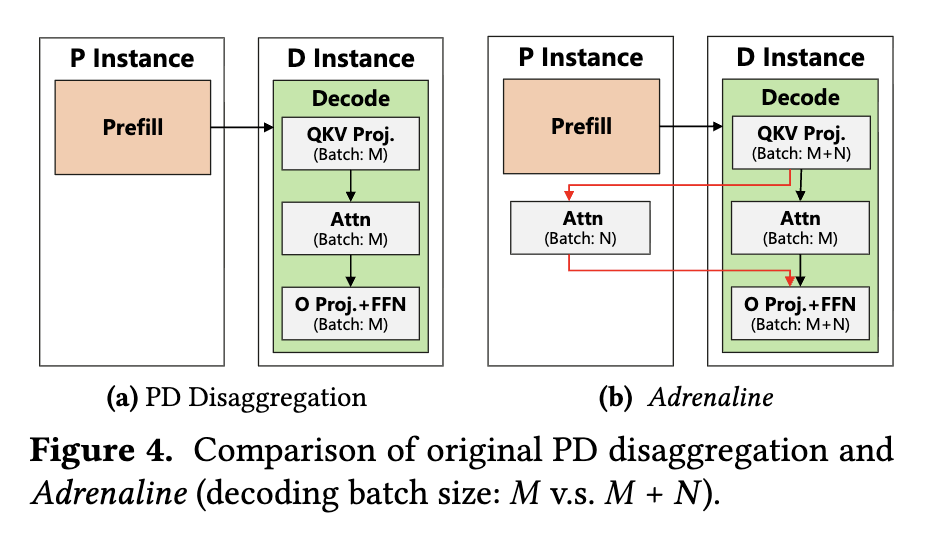
The left side is regular PD disaggregation: the Prefill instance only performs Prefill, while the Decode instance performs QKV projection, Attention, O projection, and FFN by itself, with decode batch size $M$. The right side is Adrenaline: the Decode instance still performs QKV projection, but Attention for a subset of requests (batch $N$) is offloaded to the Prefill instance. The memory and bandwidth freed on the Decode instance allow a larger batch, $M+N$. The red arrows represent Query/Attention-output transfer across instances. The transferred data is much smaller than the full KV Cache, but it lies on every decode step’s critical path.

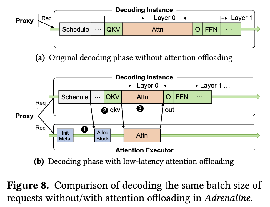
This execution-flow figure shows how offloading lands in one Decode step. Without offloading, the Decode instance executes Schedule, QKV, Attention, O, and FFN sequentially. With Attention Executor, the Decode instance allocates blocks for offloaded requests, sends compact qkv-related tensors to the Attention Executor, and receives Attention output back before continuing O projection and FFN. The key is that cross-node transfer carries relatively small Query/output tensors, not full KV Cache every step.

The labels 1-3 correspond to three optimizations Adrenaline uses to reduce synchronization overhead:

1. 1. Move metadata and memory management out of the critical path: when the Proxy decides to offload a request’s Attention, it sends the request as a hint to the Attention Executor in advance. The executor initializes runtime metadata such as prompt length, and KV cache block allocation/recycling is also prepared early. Init Meta. and Alloc Block therefore do not block every decode step.
2. 2. Aggregate QKV input transfer: Adrenaline does not send scattered $q$, $k$, and $v$ tensors separately. It aggregates the inputs required by the Attention Executor into one qkv transfer, reducing cross-instance communication count and launch overhead.
3. 3. Overlap remote and local Attention: not all Attention is offloaded; the Decode instance still runs part of Attention locally. The scheduler tries to run the remote Attention kernel on the Attention Executor at the same time as the local Attention kernel on the Decode instance. After remote Attention finishes, only out is sent back to continue O projection and FFN.

All three labels serve the same goal: move or hide metadata preparation, input transfer, and remote compute outside the critical path as much as possible. Otherwise, each layer would add a little synchronization delay and amplify TPOT.

To make this work, Adrenaline introduces three techniques:

1. Low-latency decoding synchronization: reduce the TPOT impact of cross-node Attention.
2. Resource-efficient Prefill colocation: schedule Prefill’s own work and external Decode Attention work on Prefill nodes.
3. Load-aware offloading scheduling: offload only when the benefit exceeds communication cost while preserving request SLOs.

The paper reports 2.28x higher memory-capacity utilization and 2.07x higher memory-bandwidth utilization in Prefill instances, up to 1.67x higher compute utilization in Decode instances, and 1.68x higher overall inference throughput.

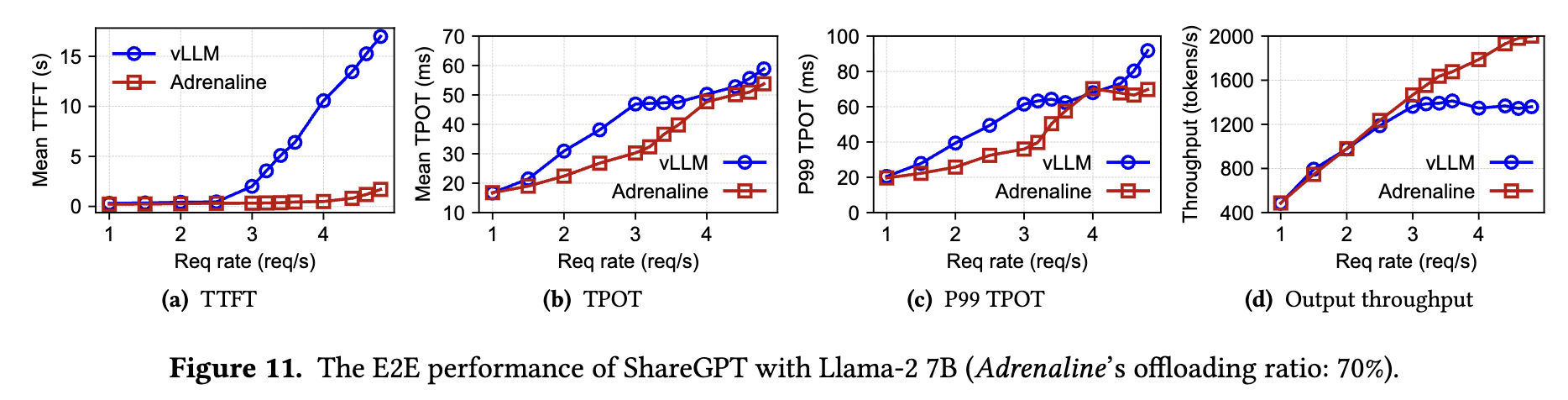
These curves show end-to-end results on ShareGPT + Llama-2 7B. The x-axis is request rate; the four subplots show mean TTFT, mean TPOT, P99 TPOT, and output throughput. As request rate increases, vLLM’s TTFT and TPOT rise earlier. By relieving Decode-side KV Cache pressure, Adrenaline maintains lower latency at higher request rates and keeps output throughput increasing. The gain depends on offloading ratio, model size, network, and workload distribution; it is not unconditional.

The limitation is also clear: every Decode step may introduce cross-node communication. Network latency, synchronization overhead, and scheduling mistakes all enter TPOT’s critical path. Adrenaline is a way to squeeze more out of a high-quality interconnect and careful scheduler, not a free lunch for every cluster.

8. Conclusion: Finer-Grained Disaggregation

The evolution of LLM Serving can be understood as repeatedly identifying and separating resource mismatches:

1. Continuous Batching / Chunked Prefill: reduce idle slots and latency spikes within a monolithic architecture.
2. PD Disaggregation (DistServe, Mooncake): separate Prefill and Decoding to optimize TTFT, TPOT, KVCache transfer, and reuse independently.
3. AE Disaggregation (MegaScale-Infer): further split Attention and Expert inside MoE Decoding to address low Expert utilization caused by sparse routing.
4. Attention Offloading (Adrenaline): after PD disaggregation, use cross-phase resource complementarity to offload Attention computation and KV Cache access.

The common theme is not “the finer the split, the better.” Disaggregation pays off only when two components have truly different resource needs, scaling strategies, or SLO targets, and when communication cost can be hidden or amortized. Longer contexts, larger MoE models, and more complex agent workloads will continue to push serving architectures toward finer-grained and more dynamic disaggregation.

References

• DistServe: Disaggregating Prefill and Decoding for Goodput-optimized Large Language Model Serving
• Mooncake: Trading More Storage for Less Computation: A KVCache-centric Architecture for Serving LLM Chatbot
• MegaScale-Infer: Serving Mixture-of-Experts at Scale with Disaggregated Expert Parallelism
• Injecting Adrenaline into LLM Serving: Boosting Resource Utilization and Throughput via Attention Disaggregation