The Evolution of Attention: From MHA to MLA and KV Cache Optimization

As the context length of Large Language Models (LLMs) continues to grow, the memory footprint of the KV Cache during inference has become the most significant bottleneck limiting model throughput and generation speed. Based on the principle that “Intra-card bandwidth > Inter-card bandwidth > Inter-node bandwidth,” an excessively large KV Cache forces the model to engage in cross-device communication, severely slowing down inference.

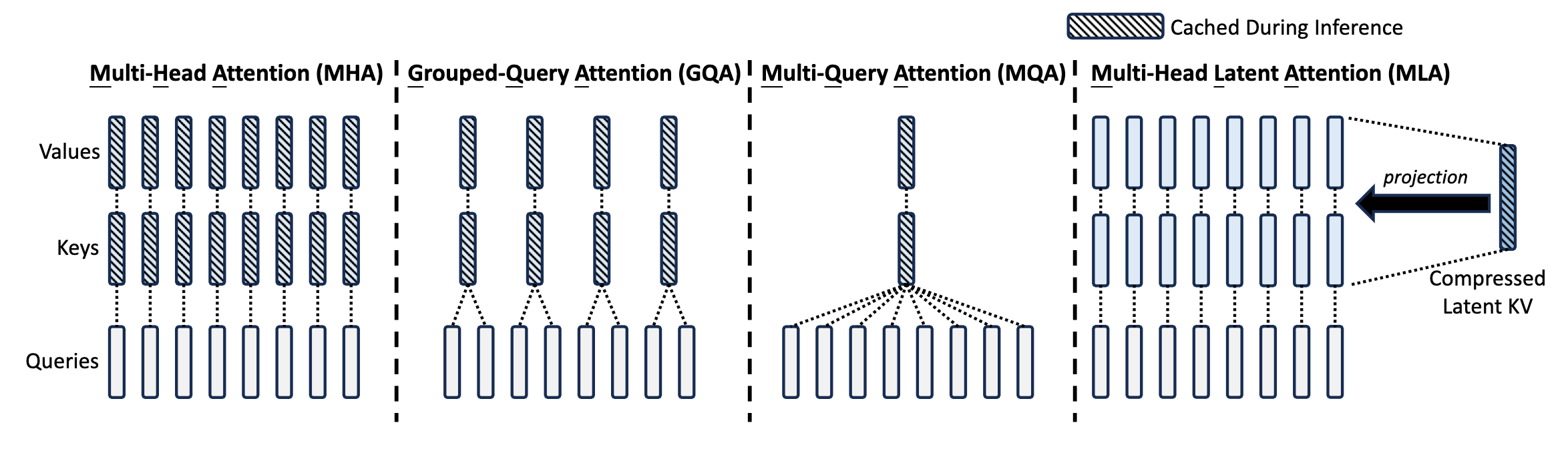
To minimize the size of the KV Cache while preserving model performance, the Attention mechanism has undergone a series of architectural evolutions. This post will walk you through the journey from MHA (Multi-Head Attention) to MQA (Multi-Query Attention), GQA (Group-Query Attention), and finally to the highly innovative MLA (Multi-head Latent Attention) proposed by DeepSeek, complete with the core mathematical derivations.

---

1. MHA (Multi-Head Attention)

MHA originated from the classic 2017 paper Attention is All You Need. Its core idea is to split the input Query (Q), Key (K), and Value (V) along the feature dimension into $h$ independent Heads. Each Head computes Attention separately, and the results are concatenated at the end.

Assume the input sequence is $\boldsymbol{x}_1, \boldsymbol{x}_2, \cdots, \boldsymbol{x}_t$. To make the mathematical expressions clear, let’s define the variables:

• $t$: The current time step (the token currently being generated).
• $i$: The index of a historical token ($i = 1, 2, \dots, t$).
• $d$: The hidden dimension of the model input.
• $h$: The total number of Attention Heads.
• $s$: The index of the specific Head being computed ($s \in [1, h]$).
• $d_k, d_v$: The dimensions of Key and Value per Head, typically $d_k = d_v = d / h$.
• $\boldsymbol{W}$: Learnable linear projection weight matrices.
• Row Vector Convention: To align with standard deep learning implementations (e.g., [batch, seq_len, hidden_dim] in PyTorch), all vector variables in this post ($\boldsymbol{x}, \boldsymbol{q}, \boldsymbol{k}, \boldsymbol{v}, \boldsymbol{c}, \boldsymbol{o}$) are defined as Row Vectors. For example, $\boldsymbol{x}_i \in \mathbb{R}^{1 \times d}$.
• Output Notation $\boldsymbol{o}_t$: The output of the Attention layer is denoted as $\boldsymbol{o}_t$ (Output), representing the context-fused feature of the current step $t$. The notation $\boldsymbol{x}_{t+1}$ is intentionally avoided here, as it typically refers to the newly predicted input token for the next autoregressive step.

The linear mapping and Attention computation for the $s$-th head are as follows:

$$ \begin{aligned} \boldsymbol{q}_i^{(s)} &= \boldsymbol{x}_i \boldsymbol{W}_q^{(s)} \in \mathbb{R}^{d_k}, & \boldsymbol{W}_q^{(s)} &\in \mathbb{R}^{d \times d_k} \\ \boldsymbol{k}_i^{(s)} &= \boldsymbol{x}_i \boldsymbol{W}_k^{(s)} \in \mathbb{R}^{d_k}, & \boldsymbol{W}_k^{(s)} &\in \mathbb{R}^{d \times d_k} \\ \boldsymbol{v}_i^{(s)} &= \boldsymbol{x}_i \boldsymbol{W}_v^{(s)} \in \mathbb{R}^{d_v}, & \boldsymbol{W}_v^{(s)} &\in \mathbb{R}^{d \times d_v} \end{aligned} $$

The $t$-th Query computes Attention with all historical Keys and Values from $1 \sim t$ (the $\sum_{i \leq t}$ denotes summing over the current and all past steps $i$):

$$ \boldsymbol{o}_t^{(s)} = \text{Attention} \left( \boldsymbol{q}_t^{(s)}, \boldsymbol{k}_{\leq t}^{(s)}, \boldsymbol{v}_{\leq t}^{(s)} \right) \triangleq \frac{\sum_{i \leq t} \exp \left( \boldsymbol{q}_t^{(s)} \boldsymbol{k}_i^{(s)\top} \right) \boldsymbol{v}_i^{(s)}}{\sum_{i \leq t} \exp \left( \boldsymbol{q}_t^{(s)} \boldsymbol{k}_i^{(s)\top} \right)} $$

Finally, the results from multiple heads are concatenated and linearly projected through an output weight matrix $\boldsymbol{W}^O$:

$$ \boldsymbol{o}_t = \text{Concat} \left( \boldsymbol{o}_t^{(1)}, \boldsymbol{o}_t^{(2)}, \cdots, \boldsymbol{o}_t^{(h)} \right) \boldsymbol{W}^O $$

During inference, to avoid redundant computations, we introduce the KV Cache, which stores the $\boldsymbol{k}_i^{(s)}$ and $\boldsymbol{v}_i^{(s)}$ of every Head for all historical tokens. This essentially trades space for time to accelerate inference.

• Pros: Each Head has its own independent K and V, providing the strongest feature representation capability and the highest upper bound for model performance.
• Cons: The size of the KV Cache scales linearly with sequence length, batch size, and the number of Heads. When processing long texts, MHA’s KV Cache consumes a massive amount of VRAM. When a single GPU cannot hold it, cross-device communication is required, severely slowing down inference.

---

2. MQA (Multi-Query Attention)

To address the exorbitant memory consumption of MHA, the 2019 paper Fast Transformer Decoding: One Write-Head is All You Need introduced MQA.

• Core Idea: All Heads share the exact same Key and Value tensors; only the Query remains independent across different Heads.
• Mathematical Expression: Notice that $\boldsymbol{k}_i$ and $\boldsymbol{v}_i$ no longer have the superscript $(s)$, meaning the concept of Heads is removed for K and V.

$$ \begin{aligned} \boldsymbol{q}_i^{(s)} &= \boldsymbol{x}_i \boldsymbol{W}_q^{(s)} \in \mathbb{R}^{d_k}, & \boldsymbol{W}_q^{(s)} &\in \mathbb{R}^{d \times d_k} \\ \boldsymbol{k}_i &= \boldsymbol{x}_i \boldsymbol{W}_k \in \mathbb{R}^{d_k}, & \boldsymbol{W}_k &\in \mathbb{R}^{d \times d_k} \\ \boldsymbol{v}_i &= \boldsymbol{x}_i \boldsymbol{W}_v \in \mathbb{R}^{d_v}, & \boldsymbol{W}_v &\in \mathbb{R}^{d \times d_v} \end{aligned} $$

• Cache Reduction: The KV Cache only needs to store the K and V for 1 Head, reducing its size to exactly $1/h$ of MHA.
• Pros: Drastically reduces VRAM consumption and accelerates inference speed.
• Cons: By aggressively compressing the representation space of K and V, the model’s overall performance (accuracy) suffers a noticeable degradation.

---

3. GQA (Group-Query Attention)

Seeking a middle ground between MHA (high performance, high memory) and MQA (low memory, lower performance), the 2023 paper GQA: Training Generalized Multi-Query Transformer Models from Multi-Head Checkpoints proposed GQA.

• Core Idea: The $h$ Heads are divided into $g$ groups. Heads within the same group share a single copy of K and V.
• Mathematical Expression: The K and V are evenly divided into $g$ groups. The superscript $([sg/h])$ indicates that the $s$-th Head is assigned to the $\lfloor sg/h \rfloor$-th K-V group. Each group’s KV is repeated $h/g$ times to satisfy the requirement of $h$ Heads.

$$ \begin{aligned} \boldsymbol{q}_i^{(s)} &= \boldsymbol{x}_i \boldsymbol{W}_q^{(s)} \in \mathbb{R}^{d_k} \\ \boldsymbol{k}_i^{([sg/h])} &= \boldsymbol{x}_i \boldsymbol{W}_k^{([sg/h])} \in \mathbb{R}^{d_k} \\ \boldsymbol{v}_i^{([sg/h])} &= \boldsymbol{x}_i \boldsymbol{W}_v^{([sg/h])} \in \mathbb{R}^{d_v} \end{aligned} $$

• Implementation Details: When $g=h$, GQA degenerates into MHA; when $g=1$, it becomes MQA. In models like LLaMA 2/3-70B, $g$ is typically set to 8. This perfectly aligns with hardware setups where each GPU handles Attention for one group of K and V, ensuring KV diversity while drastically reducing inter-card communication and VRAM usage.
• Pros: Achieves an excellent balance between inference speed and model performance.
• Cons: Requires empirical, human-defined tuning to find the optimal number of groups $g$.

---

4. MLA (Multi-head Latent Attention)

MLA is a highly innovative Attention variant introduced in DeepSeek-V2. By utilizing Low-Rank Projections, it drastically reduces the KV Cache footprint while achieving performance that even surpasses traditional MHA.

4.1 Core Idea: Low-Rank Mapping and Matrix Absorption

Instead of directly caching high-dimensional K and V tensors, MLA projects the input $\boldsymbol{x}_i$ through a low-rank matrix into a compressed latent vector $\boldsymbol{c}_i \in \mathbb{R}^{d_c}$ (shared across multiple heads):

$$ \boldsymbol{c}_i = \boldsymbol{x}_i \boldsymbol{W}_c \in \mathbb{R}^{d_c}, \quad \boldsymbol{W}_c \in \mathbb{R}^{d \times d_c} $$

Then, it uses up-projection matrices $\boldsymbol{W}_k^{(s)}$ and $\boldsymbol{W}_v^{(s)}$ to map $\boldsymbol{c}_i$ back to $\boldsymbol{k}_i^{(s)}$ and $\boldsymbol{v}_i^{(s)}$:

$$ \begin{aligned} \boldsymbol{q}_i^{(s)} &= \boldsymbol{x}_i \boldsymbol{W}_q^{(s)} \in \mathbb{R}^{d_k} \\ \boldsymbol{k}_i^{(s)} &= \boldsymbol{c}_i \boldsymbol{W}_k^{(s)} \in \mathbb{R}^{d_k}, & \boldsymbol{W}_k^{(s)} &\in \mathbb{R}^{d_c \times d_k} \\ \boldsymbol{v}_i^{(s)} &= \boldsymbol{c}_i \boldsymbol{W}_v^{(s)} \in \mathbb{R}^{d_v}, & \boldsymbol{W}_v^{(s)} &\in \mathbb{R}^{d_c \times d_v} \end{aligned} $$

• Cache Reduction: During inference, the KV Cache only needs to store this low-dimensional $\boldsymbol{c}_i$. The cache size plummets from $2 \times h \times d_k \times l$ (2 for K and V, $h$ heads, $d_k$ head dim, $l$ layers) to $d_c \times l$ (where $d_c \ll h \times d_k$).
• Matrix Absorption: You might wonder: doesn’t up-projecting $\boldsymbol{c}_i$ back into K and V at every inference step increase computation? Actually, due to the associativity of matrix multiplication, we can pre-multiply (absorb) the up-projection matrix directly into the Query’s projection matrix:

$$ \boldsymbol{q}_t^{(s)} \boldsymbol{k}_i^{(s)\top} = \left( \boldsymbol{x}_t \boldsymbol{W}_q^{(s)} \right) \left( \boldsymbol{c}_i \boldsymbol{W}_k^{(s)} \right)^\top = \boldsymbol{x}_t \left( \boldsymbol{W}_q^{(s)} \boldsymbol{W}_k^{(s)\top} \right) \boldsymbol{c}_i^\top $$

Thus, $\boldsymbol{W}_q^{(s)}$ and $\boldsymbol{W}_k^{(s)\top}$ can be merged into a single weight matrix before inference. Similarly, the Value’s up-projection matrix $\boldsymbol{W}_v^{(s)}$ can be absorbed into the final output concatenation matrix $\boldsymbol{W}^O$. Consequently, $\boldsymbol{c}_i$ participates directly in the Attention calculation, completely eliminating the need to dynamically compute K and V during inference.

(Note: In DeepSeek-V2, to save training parameters, a low-rank projection is also applied to Q as $\boldsymbol{c}'_i = \boldsymbol{x}_i \boldsymbol{W}'_c$, but this is unrelated to KV Cache optimization.)

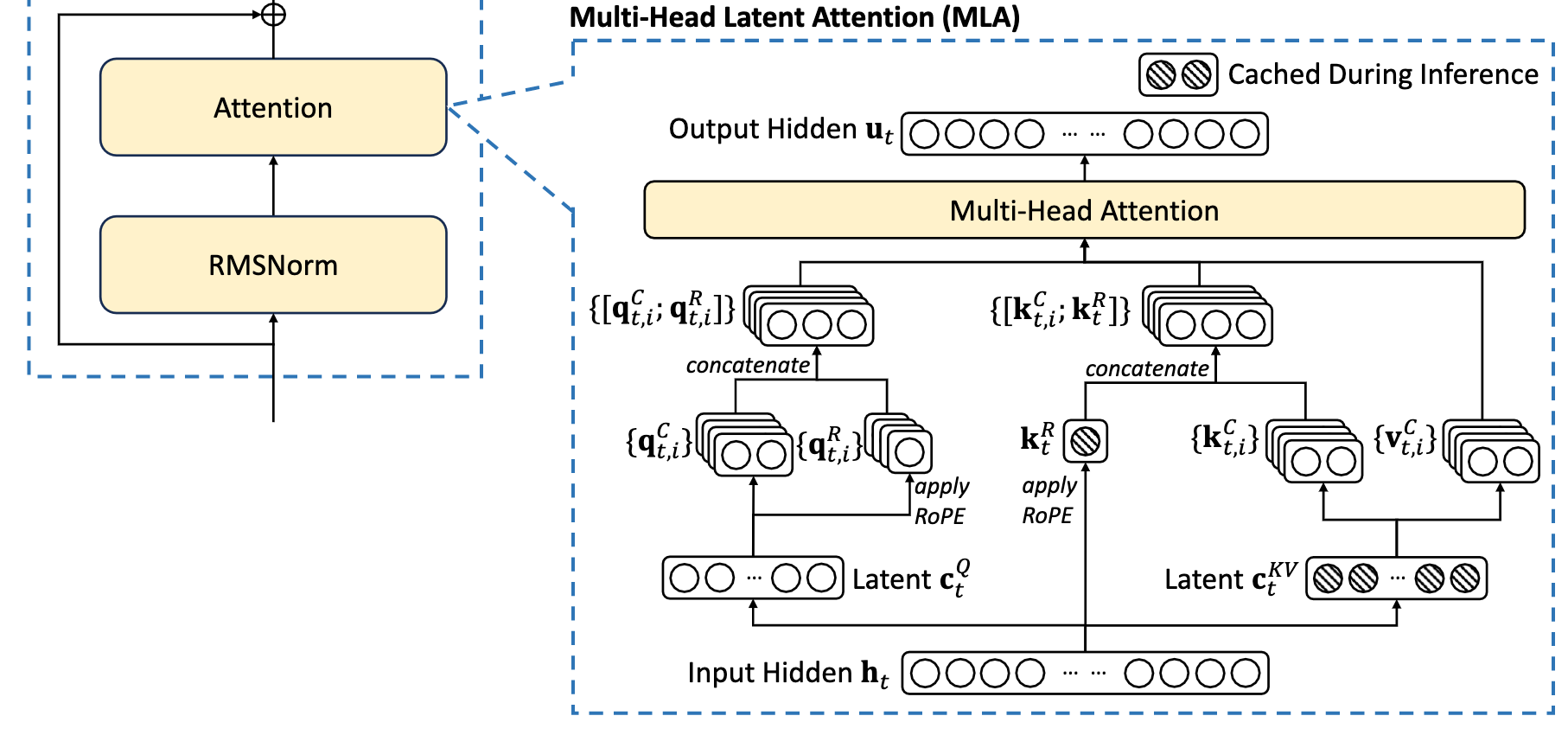
4.2 Decoupled Design for RoPE (Rotary Position Embedding) Compatibility

The matrix absorption trick has a prerequisite: there can be no interfering operations between the Q and K matrix multiplication. However, modern LLMs universally use RoPE, which inserts a rotation matrix $\boldsymbol{\mathcal{R}}$ between Q and K:

$$ \boldsymbol{q}_t^{(s)} \boldsymbol{k}_i^{(s)\top} = \left( \boldsymbol{x}_t \boldsymbol{W}_q^{(s)} \boldsymbol{\mathcal{R}}_t \right) \left( \boldsymbol{c}_i \boldsymbol{W}_k^{(s)} \boldsymbol{\mathcal{R}}_i \right)^\top = \boldsymbol{x}_t \left( \boldsymbol{W}_q^{(s)} \boldsymbol{\mathcal{R}}_{t \rightarrow i} \boldsymbol{W}_k^{(s)\top} \right) \boldsymbol{c}_i^\top $$

Because matrix multiplication is not commutative, the intervening relative position rotation matrix $\boldsymbol{\mathcal{R}}_{t \rightarrow i}$ (representing the relative positional shift from step $t$ to $i$) prevents $\boldsymbol{W}_q^{(s)}$ and $\boldsymbol{W}_k^{(s)\top}$ from being pre-absorbed.

To solve this, MLA ingeniously decouples Q and K, splitting them into a “part without RoPE” and a “part with RoPE”:

$$ \begin{aligned} \boldsymbol{q}_i^{(s)} &= \left[ \boldsymbol{c}'_i \boldsymbol{W}_{qc}^{(s)}, \boldsymbol{c}'_i \boldsymbol{W}_{qr}^{(s)} \boldsymbol{\mathcal{R}}_i \right] \in \mathbb{R}^{d_k + d_r} \\ \boldsymbol{k}_i^{(s)} &= \left[ \boldsymbol{c}_i \boldsymbol{W}_{kc}^{(s)}, \boldsymbol{x}_i \boldsymbol{W}_{kr} \boldsymbol{\mathcal{R}}_i \right] \in \mathbb{R}^{d_k + d_r} \end{aligned} $$

• Query: Contains the multi-head part without RoPE ($\boldsymbol{c}'_i \boldsymbol{W}_{qc}^{(s)}$) and the multi-head part with RoPE ($\boldsymbol{c}'_i \boldsymbol{W}_{qr}^{(s)} \boldsymbol{\mathcal{R}}_i$).
• Key: Contains the multi-head part without RoPE ($\boldsymbol{c}_i \boldsymbol{W}_{kc}^{(s)}$, up-projected from $\boldsymbol{c}_i$) and the shared part with RoPE ($\boldsymbol{x}_i \boldsymbol{W}_{kr} \boldsymbol{\mathcal{R}}_i$, generated directly from the input).

Now, the QK matrix computation becomes:

$$ \begin{aligned} \boldsymbol{q}_t^{(s)} \boldsymbol{k}_i^{(s)\top} &= \left[ \boldsymbol{c}'_t \boldsymbol{W}_{qc}^{(s)}, \boldsymbol{c}'_t \boldsymbol{W}_{qr}^{(s)} \boldsymbol{\mathcal{R}}_t \right] \left[ \boldsymbol{c}_i \boldsymbol{W}_{kc}^{(s)}, \boldsymbol{x}_i \boldsymbol{W}_{kr} \boldsymbol{\mathcal{R}}_i \right]^\top \\ &= \boldsymbol{c}'_t \left( \boldsymbol{W}_{qc}^{(s)} \boldsymbol{W}_{kc}^{(s)\top} \right) \boldsymbol{c}_i^\top + \left( \boldsymbol{c}'_t \boldsymbol{W}_{qr}^{(s)} \boldsymbol{\mathcal{R}}_t \right) \left( \boldsymbol{x}_i \boldsymbol{W}_{kr} \boldsymbol{\mathcal{R}}_i \right)^\top \end{aligned} $$

Through this decoupling, the weight matrices $\boldsymbol{W}_{qc}^{(s)} \boldsymbol{W}_{kc}^{(s)\top}$ in the first term (without RoPE) can still be perfectly absorbed!

4.3 Final KV Cache Size

In the DeepSeek-V2 configuration ($d_c = 4d_k$, $d_r = d_k / 2$), MLA ultimately only needs to cache two components:

1. The dimension-reduced latent vector $\boldsymbol{c}_i \in \mathbb{R}^{d_c}$
2. The shared RoPE key vector $\boldsymbol{k}_t^R = \boldsymbol{x}_i \boldsymbol{W}_{kr} \boldsymbol{\mathcal{R}}_i \in \mathbb{R}^{d_r}$

Its total KV Cache size is $(d_c + d_r) \times l$, roughly equivalent to 2.25 groups of GQA.

• Pros: Through low-rank projection and matrix absorption, it not only drastically reduces VRAM consumption but also surpasses traditional MHA in model performance by preserving richer joint features.
• Cons: High implementation complexity, and due to the nature of matrix absorption, the code logic differs significantly between the training and inference phases.

(Note: In the original DeepSeek paper, the notation differs slightly—e.g., the input sequence is $\mathbf{h}_t$, and the low-rank projection matrices are $\mathbf{W}^{DQ}$ and $\mathbf{W}^{DKV}$—but the core concept of decoupling and matrix absorption remains exactly the same.)

---

Conclusion

From MHA to MLA, the evolution of the Attention mechanism clearly illustrates the continuous trade-offs between algorithmic performance and engineering constraints (VRAM, bandwidth):

• MHA: High performance ceiling, but explosive KV Cache growth.
• MQA / GQA: Brute-force VRAM compression via KV sharing, at the cost of feature diversity.
• MLA: Compresses information via low-rank latent vectors, eliminates computational overhead via matrix absorption, and elegantly decouples RoPE. It ultimately achieves the “holy grail” of LLM serving: minimal VRAM footprint coupled with maximum model performance.