DeepSeek NSA and DSA: From Native Sparse Attention to Fine-Grained Token Selection

One of the core bottlenecks in long-context inference is Attention. As context length grows, Prefill has to process more historical tokens, and standard attention becomes increasingly expensive. Decoding generates only one token at a time, but every step still needs to access the ever-growing KV Cache. DeepSeek has two recent sparse-attention-related lines of work that attack this problem from different angles:

1. NSA (Native Sparse Attention): an independent sparse attention paper that emphasizes native trainability and hardware alignment. It splits attention into compression, selection, and sliding-window branches.
2. DSA (DeepSeek Sparse Attention): the sparse attention mechanism introduced in DeepSeek-V3.2 / V3.2-Exp. It is built on top of MLA and uses a Lightning Indexer to dynamically select Top-K historical KV entries for each query.

The two names are similar and the ideas overlap, but they are not the same mechanism. NSA is a more general, trainable hierarchical sparse-attention architecture. DSA is the production-oriented long-context sparsification strategy used in DeepSeek-V3.2 on top of MLA.

1. Why Is Sparse Attention Still Hard?

Full Attention is simple: each query can attend to all historical keys and values. Its expressiveness is strong, but the cost becomes problematic for long contexts:

• In Prefill, the model processes the whole sequence, and standard attention grows roughly quadratically with sequence length.
• In Decode, each new token still needs to access historical KV Cache, so per-step memory access grows with context length.
• Fixed sparse patterns, such as a sliding window, are cheap but can discard important long-range information.
• Many sparse methods reduce theoretical FLOPs, but random memory access, non-block-aligned access patterns, and unstable training can prevent real GPU speedups.

A practical sparse attention mechanism therefore needs to preserve important long-range information, remain trainable, and actually run faster on GPUs.

2. NSA: Native Sparse Attention

NSA starts from the view that sparse attention should not be a post-hoc inference patch applied to a model trained with Full Attention. Instead, it should be designed as a natively trainable attention architecture, with sparse patterns that align well with GPU block computation.

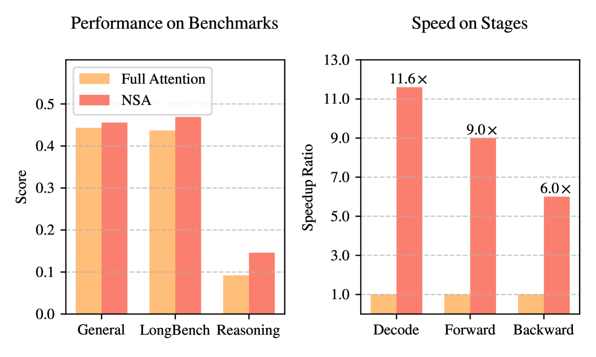
This figure answers the first question one should ask about sparse attention: is it merely faster but worse? The left side compares NSA with a Full Attention baseline across general benchmarks, long-context tasks, and reasoning evaluation. NSA does not show a clear quality drop; it is even better on average in the reported setup. The right side measures efficiency on 64K sequences across Decoding, Forward, and Backward. NSA speeds up all three, which is important because many sparse methods only help inference or only one phase. NSA is designed to help both training and deployment.

2.1 Three Attention Paths

NSA has three parallel branches: Compression, Selection, and Sliding Window.

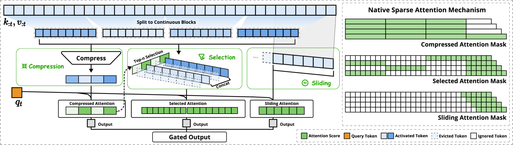
Read the figure from left to right:

1. Compression branch: compresses continuous token blocks into fewer block-level representations. It provides a coarse global view, so the model can capture long-range semantics without scanning every token.
2. Selection branch: selects important regions from historical blocks and preserves finer-grained information. It recovers details that compression might lose.
3. Sliding Window branch: always keeps a recent local window. Local context is crucial in language modeling. Without a dedicated local branch, the model may let compression or selection branches shortcut into local-pattern learning, weakening their ability to learn long-range patterns.
4. Gated Output: the three branch outputs are fused through a learned gate. Different queries can assign different weights to global compression, selected details, and local context.

The three masks on the right show the attention patterns. Green regions are where attention scores are computed, while white regions are skipped. Compression attends to compressed global blocks, Selection attends to selected important blocks, and Sliding Window attends to recent local context. NSA’s sparsity is not one fixed rule, but a combination of three views.

One core formula captures the design. Let $\mathcal{C}=\{\text{cmp},\text{slc},\text{win}\}$ denote the three branches. NSA computes a separate attention output for each branch and then combines them with learned gates:

$$ \mathbf{o}_t^*= \sum_{c\in\mathcal{C}} g_t^c\cdot \operatorname{Attn}(\mathbf{q}_t,\tilde{K}_t^c,\tilde{V}_t^c) $$

Here $\mathbf{q}_t$ is the current token’s query; $\tilde{K}_t^c,\tilde{V}_t^c$ are the keys and values constructed by branch $c$; and $g_t^c\in[0,1]$ is the gate score for that branch. The intuition is simple: instead of forcing every query to use one sparse rule, NSA lets the model allocate attention budget across global summaries, selected details, and recent local context.

Full Attention lets each query attend to all historical KV. NSA asks each branch to construct a smaller but more useful subset of KV. If the combined size of the three branches is much smaller than the full history, each query computes far fewer attention scores. The important point is that this reduction is not arbitrary pruning; it is organized around three clear roles.

To avoid symbol confusion later, keep these conventions in mind:

1. $t$ is the current query token position, and $:t$ denotes the historical prefix.
2. $c$ is one of the three branches: $\text{cmp}$, $\text{slc}$, or $\text{win}$.
3. A tilde in $\tilde{K},\tilde{V}$ means “remapped KV”, not the original full KV.
4. $g_t^c$ is the gate score that controls how much the current token relies on branch $c$.
5. The window size $w$ in NSA belongs only to the Sliding Window branch. It should not be confused with $w_{t,j}^I$ in DSA.

2.2 How Are the Three Branches Built?

The Compression branch maps continuous token blocks into block-level key/value representations. In the paper, this is done by a learnable mapping $\varphi(\cdot)$ that compresses a block of length $l$ into one compact representation. Adjacent blocks can move with stride $d$, usually with $d\lt l$, so neighboring compressed blocks overlap and less information is lost at boundaries. This branch trades token-level precision for a coarse global view.

The Compress module in the figure can be written as:

$$ \tilde{K}_t^{\text{cmp}}= \left\{ \varphi(\mathbf{k}_{id+1:id+l}) \mid 0\leq i\leq \left\lfloor\frac{t-l}{d}\right\rfloor \right\} $$

Here $i$ is the block index, $l$ is the block length, and $d$ is the stride between adjacent block starts. Thus $\mathbf{k}_{id+1:id+l}$ denotes the $i$-th continuous token block. $\varphi$ maps that block into one compressed key. The light-blue blocks under the Compression branch in the figure correspond to these compressed block representations. They are cheap because there are fewer of them, but they no longer preserve token-level detail; that is why NSA also needs Selection.

The Selection branch compensates for the details that Compression may lose. It also divides historical KV into continuous blocks, but instead of compressing every block, it scores block importance, keeps the Top-N important blocks, and feeds the fine-grained KV inside those blocks into attention. In short, Compression “thins out the global context,” while Selection “zooms in on important regions.”

Selection can be abstracted into two steps:

$$ \mathcal{I}_t= \operatorname{TopN}\left( \operatorname{score}(\mathbf{q}_t,\operatorname{blocks}(\mathbf{k}_{:t})) \right) $$$$ \tilde{K}_t^{\text{slc}}= \operatorname{Concat}\left( \{\mathbf{k}_j\mid j\in \mathcal{I}_t\} \right) $$

The first line says that the current query $\mathbf{q}_t$ scores historical blocks and selects an index set $\mathcal{I}_t$. Top-N means selecting the N highest-scoring blocks; N is the sparsity budget of the Selection branch, not the sequence length. The second line says that the original keys inside these selected blocks are concatenated and used as the input to selected attention. The green highlighted blocks in the Selection branch are precisely the selected regions. Importantly, the selection is still blockwise, not arbitrary single-token gathering, which makes it more GPU-friendly.

The Sliding Window branch keeps the most recent $w$ tokens, i.e. $\mathbf{k}_{t-w:t},\mathbf{v}_{t-w:t}$. This branch is simple but important. Local patterns often learn faster. If local context is not isolated into its own branch, the model may let Compression or Selection learn local shortcuts, weakening their ability to model long-range information. NSA separates these sources and then fuses them through gates.

Its formula is the simplest:

$$ \tilde{K}_t^{\text{win}}=\mathbf{k}_{t-w:t},\quad \tilde{V}_t^{\text{win}}=\mathbf{v}_{t-w:t} $$

This is the recent window shown in the Sliding branch. It is not meant for long-range retrieval; it guarantees that the current token always has direct access to nearby context.

2.3 Why Block-Wise?

Sparse attention cannot be judged only by theoretical complexity. GPUs prefer regular, contiguous, block-like access. If each query randomly gathers scattered tokens, the model may compute fewer scores but still lose time to gather/scatter and memory access. NSA therefore uses blockwise selection and specialized sparse kernels.

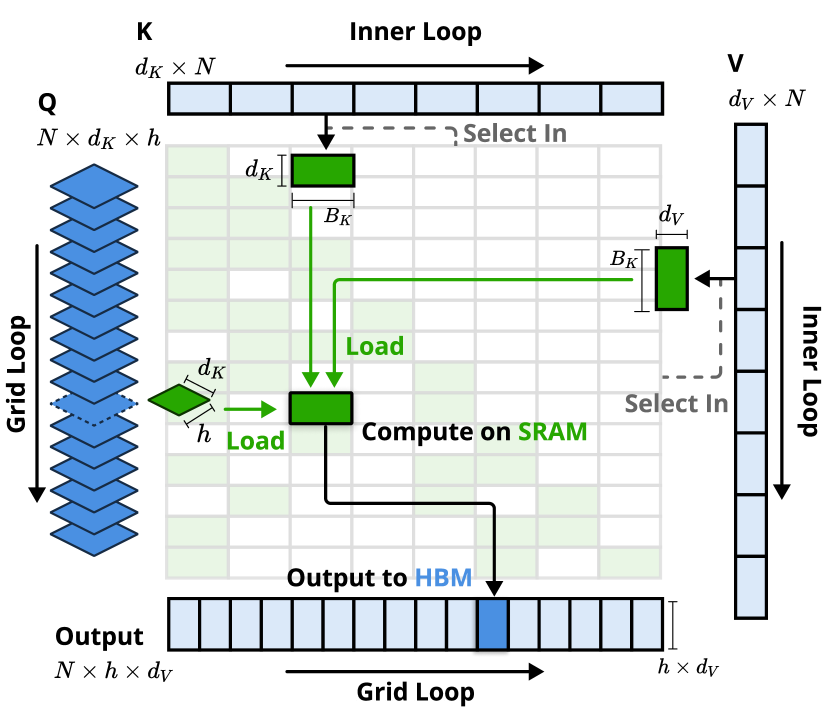
This figure shows why NSA emphasizes hardware alignment. Green blocks indicate data already in SRAM, and blue blocks indicate data in HBM. The kernel groups queries by GQA group, fetches the corresponding sparse KV blocks, and tries to finish as much attention computation as possible in SRAM. The goal is not merely to reduce FLOPs, but to reduce expensive HBM traffic and feed Tensor Cores with contiguous blocks.

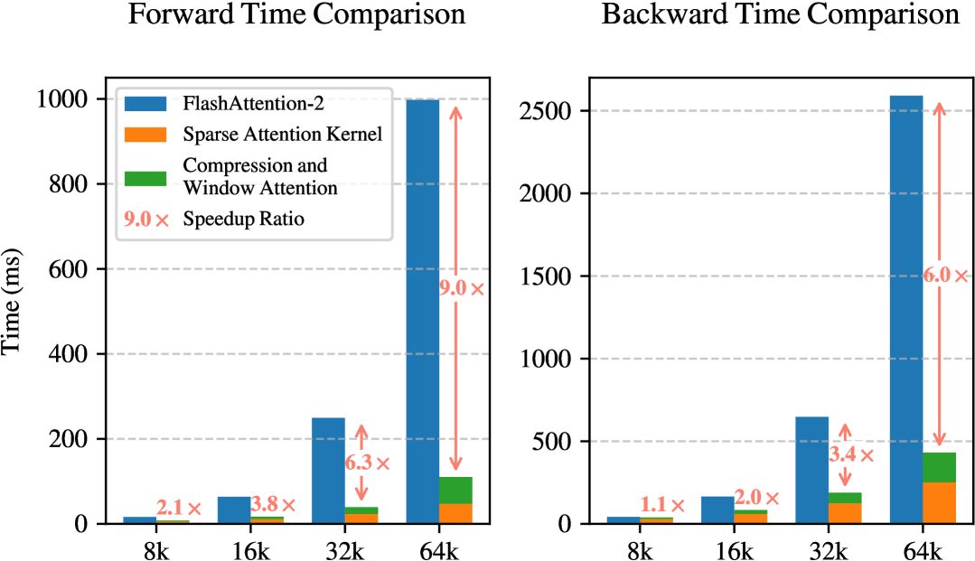
The x-axis is context length, and the y-axis is kernel latency. As the sequence gets longer, FlashAttention-2 has to cover a larger full attention region. NSA only processes sparse blocks, so its latency grows more slowly. The gap widens at longer contexts, which is exactly where sparsity matters most. The figure shows that NSA’s blockwise kernel turns theoretical sparsity into actual latency savings.

3. DSA: DeepSeek Sparse Attention

DSA is the sparse attention mechanism introduced in DeepSeek-V3.2 / V3.2-Exp. DeepSeek-V3.2 largely keeps the MoE + MLA backbone of DeepSeek-V3.1-Terminus; its key architectural change is adding DSA. Compared with NSA’s three-branch design, DSA is more focused: use a lightweight indexer to predict which historical tokens matter, then run the main attention only over Top-K historical KV entries.

3.1 DSA Relies on MLA’s Compressed KV Representation

Before DSA, it helps to understand DeepSeek’s MLA. MLA compresses key/value cache into latent representations, reducing KV Cache reads during decoding.

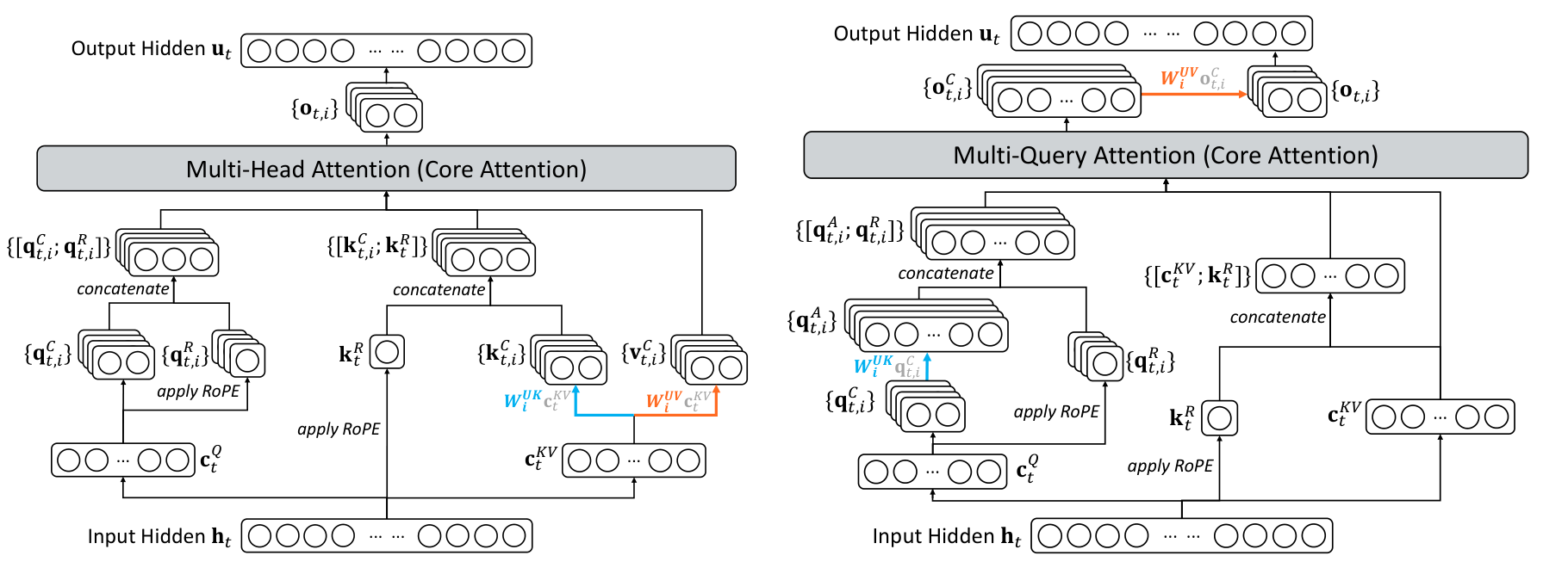
The left side shows MHA mode, and the right side shows MQA mode. MHA mode reconstructs per-head keys and values from the compressed latent representation, which is better suited for training and prefill where large matrix operations can saturate compute. MQA mode lets multiple query heads share the same latent KV entries, which is better suited for decode because decode is often constrained by KV Cache reads. Reading less KV matters more than saving a small amount of compute.

DeepSeek-V3.2 instantiates DSA on top of MLA. The technical report specifically notes that, for kernel efficiency, DSA uses the MQA mode of MLA: each latent KV entry can be shared across multiple query heads. This allows the main attention to perform sparse selection directly on compressed latent KV instead of reconstructing full per-head KV.

3.2 Lightning Indexer + Top-K Selector

DSA has three steps:

1. For the current query, the Lightning Indexer cheaply scores all historical KV entries.
2. The Top-K Selector keeps the k highest-scoring KV entries.
3. Main MLA attention runs only over those k entries.

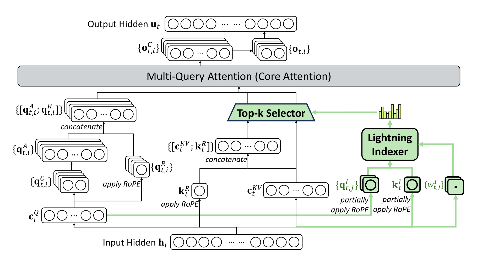
The green path is what DSA adds on top of MLA:

• Lightning Indexer receives query-related features and historical key-related features, then outputs an index score for each historical position.
• Top-K Selector selects the most relevant KV entries according to those scores.
• Core Attention no longer attends to all historical KV, but only to the selected Top-K set using Multi-Query Attention.

The Lightning Indexer first answers a cheap question: “Which historical positions are likely to matter for the current query?” Before reading its score formula, follow the green data path in the architecture figure:

1. Input Hidden at the bottom is the input hidden state of the current layer. Let $\mathbf{h}_t\in\mathbb{R}^d$ denote the hidden state at the current position $t$, and let $\mathbf{h}_s\in\mathbb{R}^d$ denote the hidden state that historical position $s$ had when it entered this layer.
2. The current $\mathbf{h}_t$ goes through a lightweight query-side projection, producing $H^I$ indexer query vectors and $H^I$ head weights. Abstractly:

$$ \left(\{\mathbf{q}_{t,j}^I\}_{j=1}^{H^I}, \{w_{t,j}^I\}_{j=1}^{H^I}\right) =f_Q^I(\mathbf{h}_t) $$

3. When each historical token reaches this layer, its $\mathbf{h}_s$ goes through a key-side projection to produce one indexer key:

$$ \mathbf{k}_s^I=f_K^I(\mathbf{h}_s) $$

The $\mathbf{k}_s^I$ produced at every position is stored in a small indexer key cache dedicated to the layer. At decode position $t$, the system does not need to keep or recompute all historical hidden states; it only reads the indexer keys cached before position $t$, namely $\mathbf{k}_1^I,\mathbf{k}_2^I,\ldots,\mathbf{k}_{t-1}^I$.

$f_Q^I$ and $f_K^I$ are abstract notation used here to make the variable origins explicit; they are not additional equations introduced by the paper. In the implementation, the query-side path also reuses MLA’s low-rank query latent.

The Lightning Indexer is a small multi-head scoring module rather than a single-head scorer. In the public DeepSeek-V3.2 configuration, index_n_heads=64 and index_head_dim=128: it uses 64 low-dimensional query heads to evaluate historical relevance from different subspaces, while all heads compare against the same shared indexer key. This is MQA-like: multiple query perspectives share one key representation, increasing scoring capacity without caching 64 indexer keys per historical token.

Once the current query-side $\mathbf{q}_{t,j}^I,w_{t,j}^I$ and the historical key cache are available, the technical report writes the index score as:

$$ I_{t,s}= \sum_{j=1}^{H^I} w_{t,j}^I\cdot \operatorname{ReLU}\left( \mathbf{q}_{t,j}^I\cdot \mathbf{k}_s^I \right) $$

Here $j$ ranges over the $H^I$ indexer query heads, with $H^I=64$ in the public configuration. Both $\mathbf{q}_{t,j}^I$ and $\mathbf{k}_s^I$ lie in $\mathbb{R}^{d^I}$, with $d^I=128$ publicly configured. The superscript $I$ marks quantities belonging to the Indexer, not the main MLA attention.

For each historical position $s$, query head $j$ computes $\mathbf{q}_{t,j}^I\cdot\mathbf{k}_s^I$. The heads share the same $\mathbf{k}_s^I$, but their different query projections still measure relevance from different perspectives. ReLU discards negative matches, and $w_{t,j}^I$ dynamically combines the positive evidence across heads. This weight is also produced from the current $\mathbf{h}_t$ through $f_Q^I$; it is neither a manually fixed constant nor the NSA sliding-window size $w$.

The whole formula therefore means: the Lightning Indexer uses multiple low-dimensional heads to score historical position $s$ from different perspectives, ReLU keeps only positive evidence, and $w_{t,j}^I$ combines these head-level scores into the final index score $I_{t,s}$. The higher $I_{t,s}$ is, the more likely position $s$ is to enter Top-K. The goal is not to reproduce the full main attention computation exactly, but to build a cheap pre-filter that finds promising KV candidates for the expensive attention to process.

After obtaining all $I_{t,s}$, DSA keeps the Top-K positions:

$$ \mathcal{S}_t= \{s\mid I_{t,s}\in \operatorname{TopK}(I_{t,:})\} $$

The main attention output is computed only over this selected set:

$$ \mathbf{u}_t= \operatorname{Attn} \left( \mathbf{h}_t, \{\mathbf{c}_s\mid s\in \mathcal{S}_t\} \right) $$

Here $\mathbf{h}_t$ is the current hidden state, and $\mathbf{c}_s$ is the latent KV entry cached by MLA. The Lightning Indexer still scans historical candidates, but it is a lightweight scorer. The expensive main MLA attention is restricted to $\mathcal{S}_t$.

If the sequence length is $L$ and each query selects $k$ historical tokens, the main attention complexity drops from roughly $O(L^2)$ to $O(Lk)$. Here $k$ is the Top-K selection budget, not the key vector. In DeepSeek-V3.2-related materials, the common setting is index_topk=2048. For a 128K context, 2048 is only about 1.6% of the sequence.

DSA does not ignore global context. The indexer still considers all previous tokens. The difference is that the expensive attention is only applied to the learned important subset.

3.3 How Is the Indexer Trained?

DSA is not a hand-coded Top-K rule. It trains an indexer to mimic the selection preference of the main attention. The report describes two stages.

The first stage is Dense Warm-up. Dense attention is still used, the main model is frozen, and only the Lightning Indexer is trained. The dense attention distribution is used as a teacher: its scores are aggregated and normalized into a target distribution, and the indexer is trained with a KL-divergence loss to match that distribution. Intuitively, this teaches the indexer: “If full attention looked at every historical token, which positions would it care about?”

The objective is:

$$ \mathcal{L}^I= \sum_t \mathbb{D}_{\mathrm{KL}} \left( p_{t,:}\;\middle\|\; \operatorname{Softmax}(I_{t,:}) \right) $$

Here $p_{t,:}$ is the teacher distribution aggregated from dense attention, while $\operatorname{Softmax}(I_{t,:})$ is the distribution produced by the Lightning Indexer over all historical positions. A smaller KL divergence means the indexer better matches full attention’s preference. In the architecture figure, the Lightning Indexer is not yet deciding the sparse path at this stage; it is first learning how to score like the main attention.

The second stage is Sparse Training. Top-K selection is enabled, and the main model adapts to the sparse attention pattern. The indexer still aligns with the main attention preference, but now only on the selected token set. The main model learns through language modeling loss, while the indexer learns ranking through its own alignment loss.

After Top-K is enabled, the alignment is computed only on the selected set $\mathcal{S}_t$:

$$ \mathcal{L}^I= \sum_t \mathbb{D}_{\mathrm{KL}} \left( p_{t,\mathcal{S}_t}\;\middle\|\; \operatorname{Softmax}(I_{t,\mathcal{S}_t}) \right) $$

This corresponds to the Top-k Selector in the figure: only KV entries in $\mathcal{S}_t$ enter the main attention, so the indexer must learn to rank well inside that subset. Meanwhile, the main model adapts through the language modeling loss to the fact that it can only attend to Top-K entries.

The important point is that DSA is not simply truncating full attention into Top-K. It first trains the indexer to imitate dense attention preferences, and then trains the model and selector together under the sparse pattern. Without this adaptation, the Top-K selector could miss important tokens early in training and degrade model quality.

3.4 DSA’s Cost Impact

The DeepSeek-V3.2 technical report compares inference cost with DeepSeek-V3.1-Terminus. The following figures show Prefill and Decode cost as token position grows.

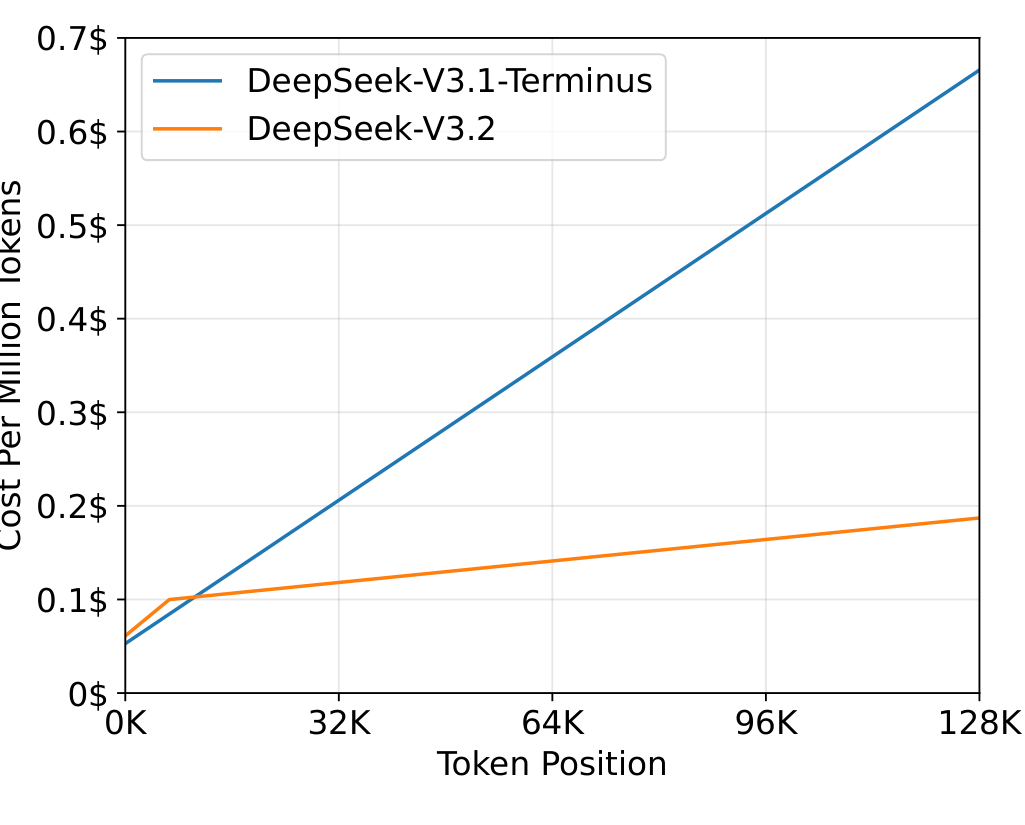
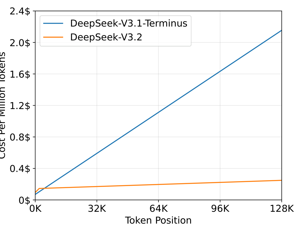
The important part is the slope at long context. The blue line is DeepSeek-V3.1-Terminus and the orange line is DeepSeek-V3.2. In the Prefill plot, the blue line rises clearly with token position, meaning long-sequence prefill becomes increasingly expensive. The orange line grows much more slowly, showing that DSA suppresses the attention cost growth. In the Decode plot, the difference is even clearer: the blue line becomes almost linearly more expensive as position grows, while the orange line stays at a much lower slope.

DSA does not eliminate KV Cache, and the indexer is not free. It changes the cost structure: the cheap Lightning Indexer still scans globally, but the expensive main attention only attends to a learned Top-K subset. The longer the context, the more valuable this replacement becomes.

4. NSA and DSA: Relationship and Differences

NSA and DSA both ask the same question: Does every query really need to attend to the full history in long-context modeling? Both answer no, but they implement sparsity differently.

Dimension	NSA	DSA
Source	Native Sparse Attention paper	DeepSeek-V3.2 / V3.2-Exp technical report
Sparsity granularity	More block-wise and hierarchical	More token-wise / KV-entry Top-K
Core design	Compression + Selection + Sliding Window	Lightning Indexer + Top-K Selector + sparse MLA
Dependency on MLA	No, it is a general sparse attention architecture	Yes, DeepSeek-V3.2 instantiates it under MLA/MQA mode
Training perspective	Emphasizes native trainability and backward kernels	Continued training adapts the indexer and the main model
Hardware focus	Blockwise sparse kernels, Tensor Core / SRAM friendliness	Indexer, Top-K, sparse MLA / FlashMLA-style path

NSA can be understood as a hierarchical sparse attention architecture: coarse compression preserves global context, fine-grained selection preserves important details, and sliding window preserves local context. Its sparse pattern is more structured and more naturally compatible with blockwise kernels.

DSA is more like a dynamic token selector on top of MLA: each query selects Top-K historical KV entries based on content. Its advantage is fine-grained, content-dependent selection; its cost is that Top-K and sparse gather place higher demands on kernels, cache locality, and scheduling.

5. When Should We Care About NSA vs DSA?

From a research and architecture-design perspective, NSA is especially interesting. It systematically addresses why sparse attention should be natively trainable, why it should be blockwise, why it needs three branches, and how forward/backward can both be accelerated.

From the perspective of current DeepSeek model deployment, DSA is more direct. DeepSeek-V3.2 uses DSA: it adds Lightning Indexer and Top-K token selection to an existing MLA backbone, aiming to substantially reduce long-context prefill and decode cost while preserving model quality.

The shared lesson is that future long-context models will not rely only on larger KV Cache or more memory. A more likely direction is to let the model learn which historical information the current token really needs, while making the selection process hardware-friendly enough to run at scale.

References

• Native Sparse Attention: Hardware-Aligned and Natively Trainable Sparse Attention
• DeepSeek-V3.2: Pushing the Frontier of Open Large Language Models
• DeepSeek-V3.2 Model Documentation
• DeepSeek Sparse Attention (DSA) — NVIDIA cuDNN