SoCC'20 | InferLine: latency-aware provisioning and scaling for prediction serving pipelines

Overview

This paper introduces InferLine, a system for provisioning and managing each stage of prediction pipelines to meet end-to-end tail latency constraints while minimizing cost. InferLine consists of a low-frequency combinatorial planner and a high-frequency auto-scaling tuner. The Planner leverages stage profiling, discrete event simulation, and constrained combinatorial search to automatically select hardware types, replicas, and batching parameters for each stage in the pipeline. The Tuner uses network calculus to auto-scale each stage to meet tail latency objectives, thereby responding to changes in query arrival processes. This paper demonstrates that InferLine reduces cost by 7.6x compared to existing methods while having a 34.5x lower latency SLO miss rate on real workloads, and is generalized in state-of-the-art model serving frameworks.

Research Background

Background

Prediction pipelines combine multiple machine learning models and data transformations to support complex prediction tasks. For example, state-of-the-art visual question answering services combine language models with vision models to answer questions. Prediction pipelines can be represented as directed acyclic graphs (DAGs), where each vertex corresponds to a model (e.g., mapping images to objects in the image) or data transformation (e.g., extracting keyframes from video), and edges represent data flow between vertices.

This paper studies several representative pipelines (Figure 2). The image processing pipeline includes basic image preprocessing (e.g., cropping and resizing), followed by using deep neural networks for image classification. The video surveillance pipeline uses object detection models to identify vehicles and people, then performs subsequent analysis on any relevant images, including vehicle and person identification and license plate extraction. The social media pipeline combines computer vision models with multi-stage language models to translate and classify posts based on text and linked images, identifying source language and translating posts when necessary. The TensorFlow (TF) cascade pipeline combines fast and slow TensorFlow models, invoking the slow model only when necessary.

Challenges

Prediction pipelines pose new challenges to the design and provisioning of prediction serving systems. This paper first discusses how the addition of specialized hardware accelerators and the need to meet end-to-end latency constraints lead to a combinatorial configuration space. This paper then discusses some of the complexities of meeting tail latency SLOs under bursty random query loads. This paper subsequently contrasts this work with perspectives from the data flow processing literature, which has some structural similarities but targets fundamentally different applications and performance goals.

Combinatorial Configuration Space

1. Many machine learning models can be compute-intensive with significant parallelization opportunities. In some cases, this parallelism can lead to orders of magnitude improvements in throughput and latency. For example, TensorFlow can perform predictions on the relatively large ResNet152 neural network at 0.6 queries per second (QPS) on CPU and 50.6 QPS on NVIDIA Tesla K80 GPU, an 84x throughput difference. However, not all models benefit equally from hardware accelerators. For example, decision trees have little parallelization space and are difficult to accelerate with GPUs.

2. In many cases, to fully utilize available parallel hardware, queries must be batched (e.g., ResNet152 requires a batch size of 32 to maximize throughput on K80). However, batching queries also increases latency. The choice of maximum batch size depends on the hardware and model and affects the end-to-end latency of the pipeline.

3. In heavy query load settings, it is often necessary to replicate individual operators in the pipeline to provide the throughput required by the workload. When we scale the pipeline through replication, each operator scales differently, and this effect is amplified by using conditional control flow in the pipeline, causing some components to be queried more frequently than others. Low-cost configurations require fine-grained scaling for each operator.

Allocating parallel hardware resources to individual models creates a complex model-dependent trade-off space between cost, throughput, and latency. This trade-off space grows exponentially with each model in the prediction pipeline. In one stage of the pipeline, decisions about hardware selection, batching parameters, and replication factors affect the feasible choice set for other stages, as end-to-end latency constraints need to be satisfied. For example, in one model, trading latency for increased throughput by increasing batch size can reduce the latency budget for other models in the pipeline, thus also limiting feasible hardware configurations.

Queuing Delay

Due to resource and model heterogeneity, different stages of the pipeline may run at different speeds, so each stage requires a queue. Queues also allow absorption of irregularities in query arrival intervals and can be an important component of end-to-end latency. During pipeline configuration, queuing delay must be explicitly considered as it directly depends on the relationship between the arrival interval process and the system configuration.

Random and Unpredictable Workloads

Prediction serving systems must respond to bursty, random query streams. At a high level, these random processes are characterized by their mean arrival rate λ and coefficient of variation, a dimensionless variability measure defined as $CV_A^2=σ2/μ2$, where $μ=1/λ$ and $σ$ are the mean and standard deviation of query arrival times. Processes with higher $CV_A^2$ have higher variability and typically require additional over-provisioning to meet latency objectives. Clearly, over-provisioning the entire pipeline on specialized hardware can be very expensive. Therefore, being able to identify and configure bottlenecks in the pipeline to accommodate bursty arrival processes is crucial. Finally, as workloads change, we need mechanisms to monitor, quickly detect, and tune each stage in the pipeline.

Comparison with Stream Processing Systems

Many challenges regarding configuring and scaling pipelines have been studied in the context of general-purpose data flow processing systems. However, these systems are primarily dedicated to supporting more traditional data processing workloads, including stateful aggregation operators and support for various windowing operations. These systems tend to maximize throughput while avoiding backpressure, treating latency as a secondary performance goal, without considering tail latency.

• This method’s SLO target is P99 tail latency.

Method Introduction

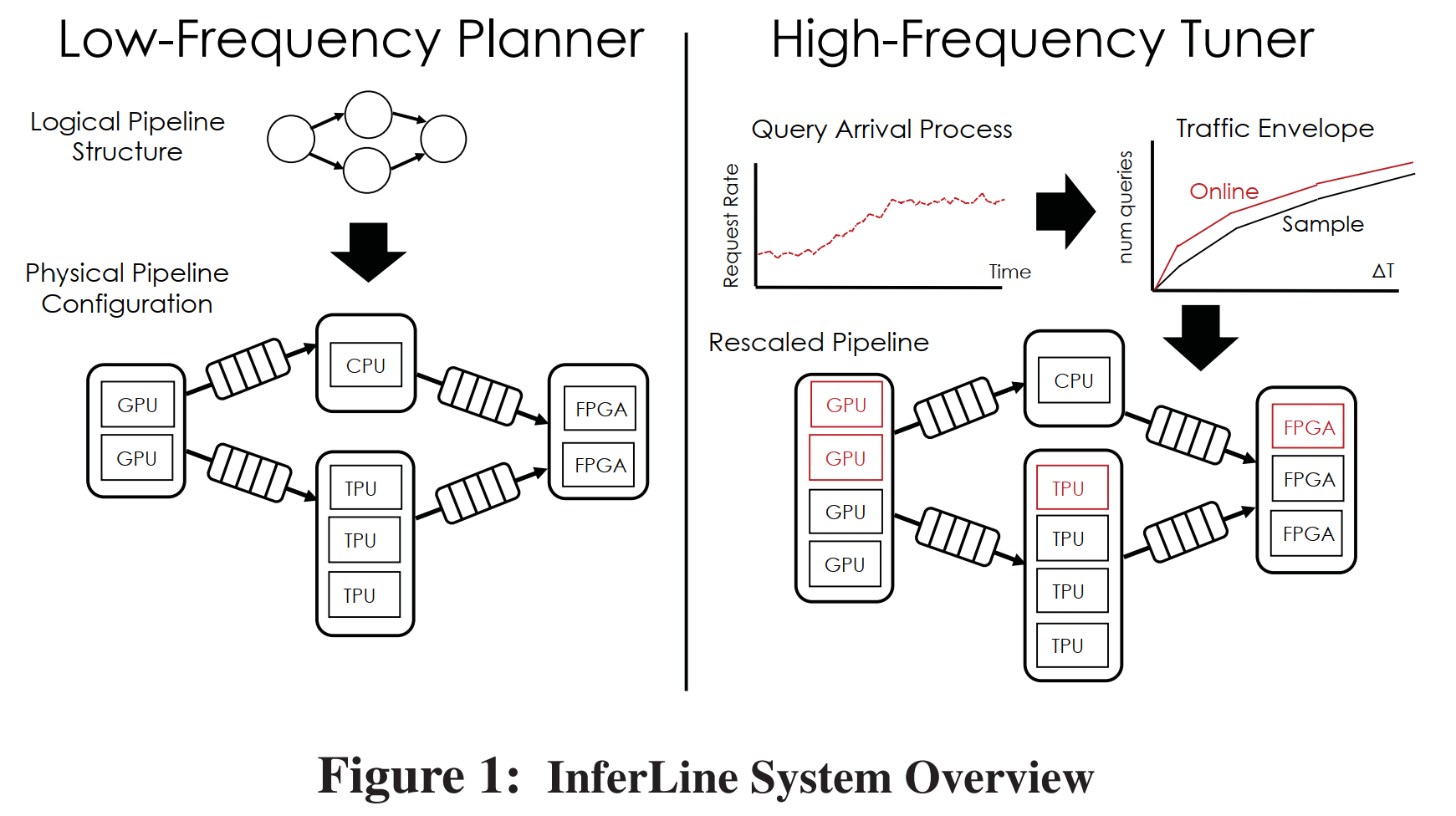
This paper designs a system called InferLine. InferLine requires an infrequently operated planner (Low-Frequency Planning) to reconfigure the entire pipeline, and a tuner (High-Frequency Tuning) to dynamically observe query traffic and adjust pipeline configurations.

InferLine can run on top of any prediction serving system, but these systems need to meet certain requirements. The underlying serving system must be able to:

1. Deploy multiple replicas of a model and have the ability to scale the number of replicas in a cluster;
2. Allow batched inference and be able to configure maximum batch size;
3. Use a centralized batch queuing system to distribute batches among model replicas.

The first two properties are necessary for InferLine’s configuration serving engine, and the centralized queuing system provides deterministic queuing behavior that can be accurately simulated by the estimator. In this paper’s experimental evaluation, InferLine runs with Clipper and TensorFlow Serving. Both systems can meet these requirements with only minor modifications.

To deploy a new prediction pipeline managed by InferLine, developers provide a driver, sample query traces for planning, and a latency service level objective (SLO). The driver function interleaves application-specific code with asynchronous calls to models hosted in the underlying serving system to execute the pipeline.

Low-Frequency Planning

Profiler

When the plan is executed for the first time, InferLine uses the Profiler to create performance profiles for all individual models referenced by the driver. Performance profiles determine model throughput through functions parameterized by hardware type and maximum batch size. Entries in model files are measured empirically by individually evaluating models in a given configuration using queries from sample traces. Individual model configurations correspond to specific values for each parameter and the model’s replication factor. Because models scale horizontally, profiling a single replica is sufficient. Profiling for each hardware and batch size pair only needs to be performed once and is reused in subsequent Planner runs.

Estimator

The Estimator is responsible for quickly estimating the end-to-end latency for a given pipeline configuration on sample query traces. It takes pipeline configuration, individual model profiles, and sample traces of query workload as input, and returns accurate estimates of latency for each query in the trace. The Estimator is implemented as a continuous-time discrete event simulator [5], simulating the entire pipeline, including queuing delays and conditional control flow (using scale factor s). The Estimator maintains a global logical clock that advances from one discrete event to the next, with each event triggering future events processed in chronological order. Because the simulation only models discrete events, it can accurately simulate hours of real-world traces in hundreds of milliseconds.

The Estimator simulates the deterministic behavior of queries through a centralized batch queuing system. It combines this with model profile information, which informs the simulator how long it takes for a model running on a specific hardware configuration to process a batch of a given size.

Planning Algorithm

The Planner finds a cost-effective initial pipeline configuration based on end-to-end latency SLO and specified arrival process. It uses a globally aware, cost-minimizing optimization algorithm to set three control parameters for each model in the pipeline. At each iteration of the optimization algorithm, the planner uses model profiles to select cost-minimizing steps while relying on the estimator to check for latency constraint violations. After generating the initial configuration and deploying the pipeline to serve live traffic, the planner will periodically (hours to days) rerun on recent arrival history to find the cost-optimal configuration for the current workload.

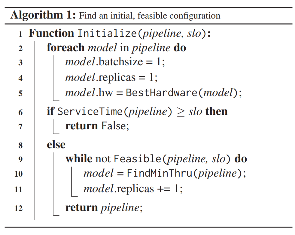
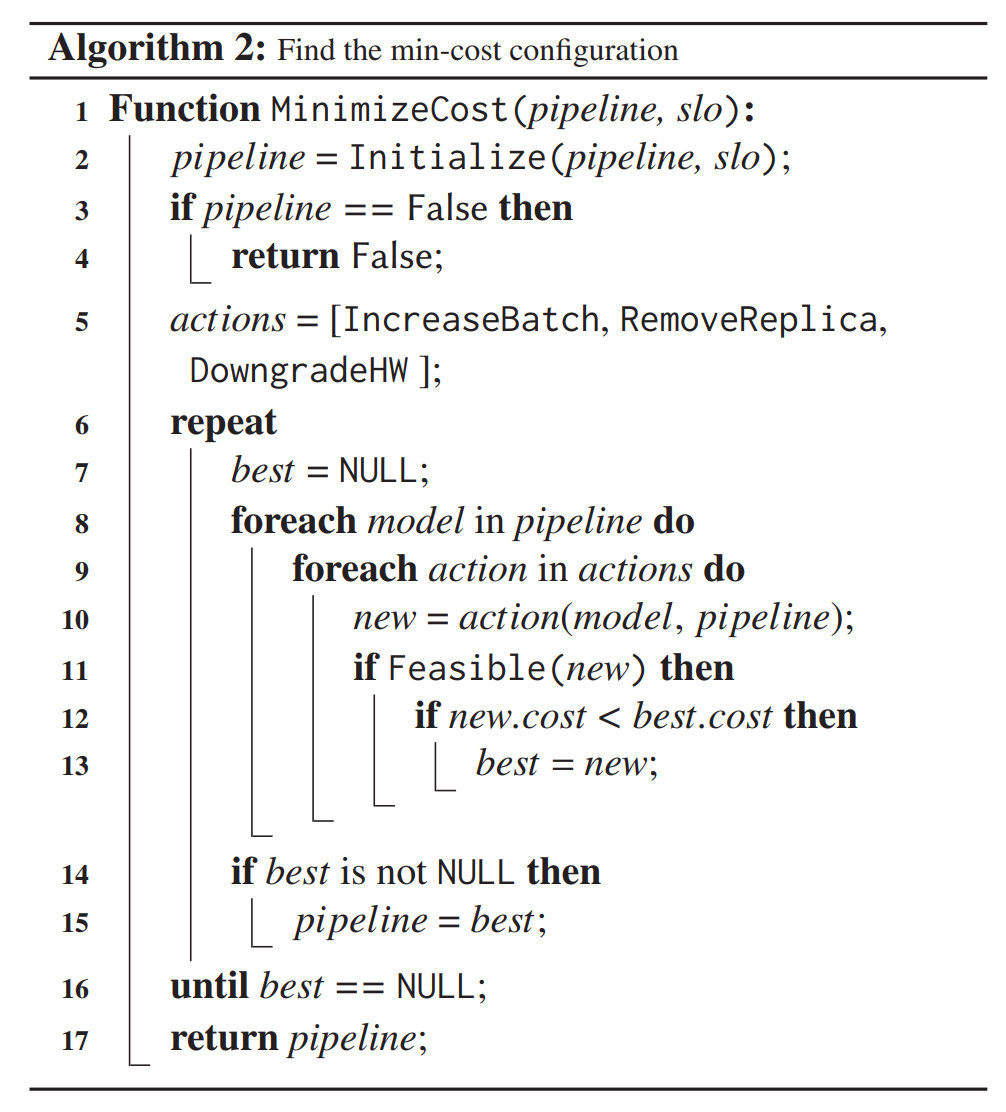
At a high level, the planning algorithm is an iterative constrained optimization process that greedily minimizes cost while ensuring latency constraints are satisfied. The algorithm is divided into two phases. In the first algorithm (Algorithm 1), a feasible initial configuration that satisfies the latency SLO is found while ignoring cost. In the second algorithm (Algorithm 2), it greedily modifies the configuration to reduce cost while using the estimator to identify and reject configurations that violate the latency SLO. The algorithm converges when no cost-reducing modifications can be made to the configuration without violating the SLO.

Algorithm 1: Initialize a Feasible Configuration

1. First, set the input batch size of each model in the pipeline to 1, set no replicas, and choose the best hardware for the model.
2. ServiceTime is the lower bound of latency that can be achieved with current hardware (assuming each model in the pipeline is deployed on dedicated, optimal hardware, the time required to execute a single request. Therefore, the relationship exists: service time <= any end-to-end latency; when service time > SLO, there must be 100% end-to-end latencies > SLO). If ServiceTime is greater than or equal to SLO, configuration cannot proceed.
3. If ServiceTime is less than SLO, determine whether the pipeline is now feasible (meets tail latency target). If not satisfied, find the bottleneck model in the pipeline, increase replicas for that model so that throughput at this point increases. Repeat this process until the configuration is feasible.
4. Return the feasible pipeline configuration.

Algorithm 2: Find the Lowest Cost Configuration

1. First, use Algorithm 1 to find a feasible configuration; if not found, abort directly.
2. Define three possible operations: increase batch size, remove model replica, downgrade hardware.
3. For each model in the pipeline, try the three operations from point 2. If these operations can be performed (reducing pipeline cost), execute the operation until no operation can be performed on all models.
4. Return the current greedily found minimum cost pipeline.

High-Frequency Tuning

The Tuner monitors the dynamic behavior of the arrival process to adjust the replication factor for each model and maintain high SLO achievement at low cost. InferLine only adjusts the replication factor for each model during tuning to avoid expensive hardware migration operations during live serving and ensure rapid scaling decisions can be made to maintain latency SLO (P99 latency), even during sharp bursts. The Tuner continuously monitors the current service envelope to simultaneously detect deviations from the planned trace service envelope at different time scales. By analyzing the time scale at which deviations occur, the Tuner can take appropriate mitigation measures within seconds to ensure SLO requirements are met without unnecessarily increasing cost. It ensures latency SLO is maintained during unexpected changes to arrival workload during Planner runs.

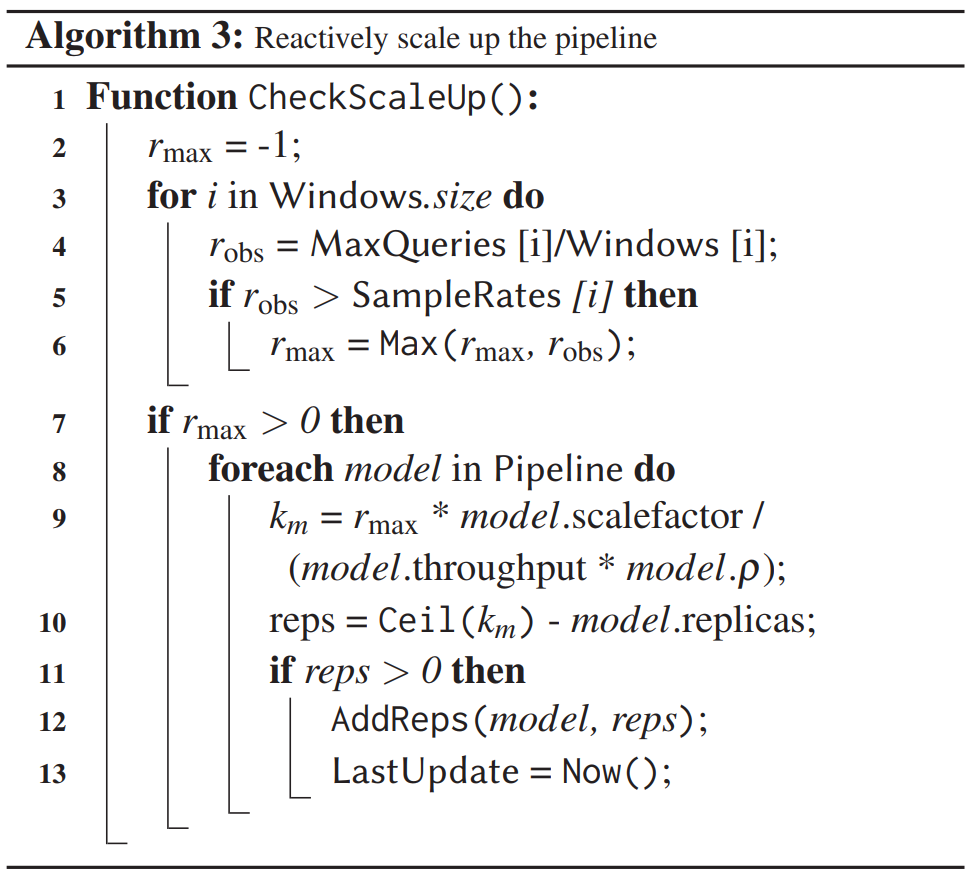
Algorithm 3: Reactively Scale Pipeline

1. Set a certain number of time windows of different sizes, iterate through different window sizes (line 3): For a certain size time window (Windows.size), slide on the timeline to find the maximum arrival rate for that time window (MaxQueries [i]/Windows [i]) (line 4) and compare with the sample arrival rate (SampleRates) for that window size. If the condition is met: “the maximum arrival rate is greater than the sample arrival rate for the same window size” (line 5), record the maximum arrival rate that satisfies this condition for different time windows. (line 6)
2. To determine how to reset the pipeline, the Tuner calculates the number of replicas required for each model to process $r_{max}$, i.e., $k_m=\lceil\frac{r_{max}*s_m}{μ*ρ_m} \rceil$ (lines 9-10). $s_m$ is the scale factor for model m (the proportion of conditional branches in the pipeline pointing to model m), which prevents over-provisioning for models that only receive partial queries due to conditional logic. $ρ_m$ is the maximum supply ratio, which ensures sufficient redundancy in the model to handle bursts.
3. Using the results calculated in step 2, add replicas for each model.

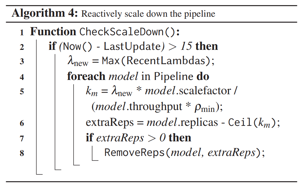
Algorithm 4: Reactively Scale Down Pipeline

1. Determine whether 15 seconds have passed since the current time since the last update, to avoid oscillating configuration changes.
2. Using the same method as Algorithm 3, find the most recent arrival rate, then remove some unnecessary replicas for each model.

Experimental Results

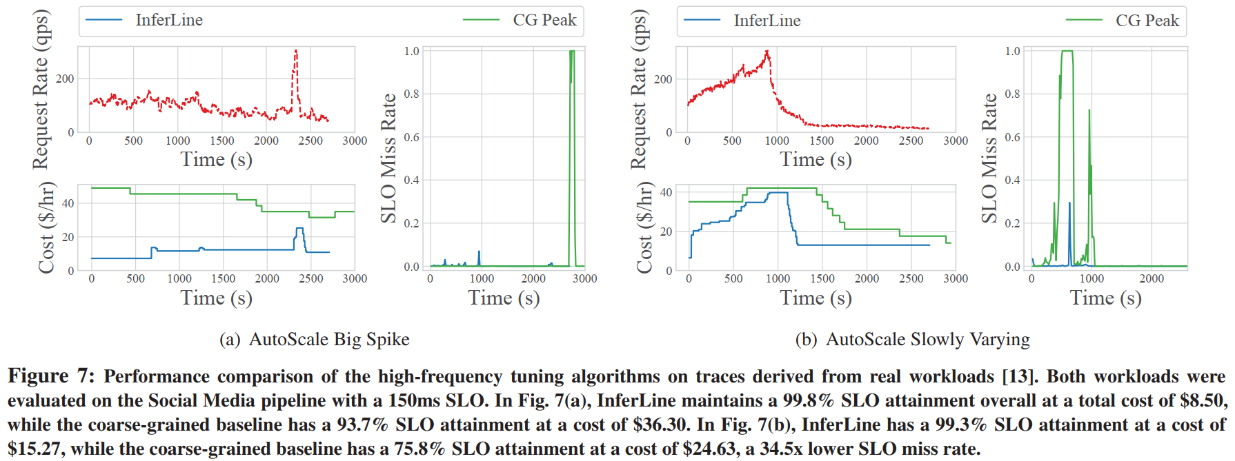
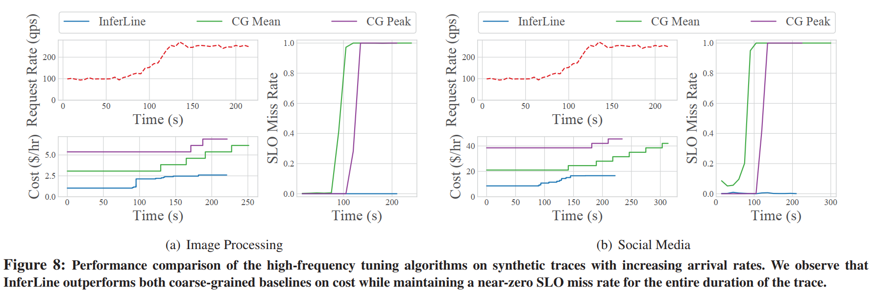
From the above three figures, it can be seen that InferLine achieves a lower P99 miss rate at lower cost compared to CG-Mean and CG-Peak.

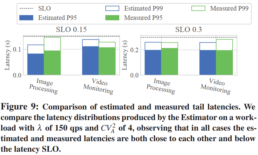
Figure 9 above shows that in all four experiments, estimated and measured P99 latencies are close. Additionally, the estimator has the critical property of ensuring P99 latency for feasible configurations is below the latency target. The near-zero SLO miss rate in Figure 6 is further evidence of the estimator’s ability to detect infeasible configurations.

Figure 10 above shows the Planner’s sensitivity:

1. Cost decreases as SLO (P99 tail latency) increases
2. More bursty workloads require higher cost configurations
3. Cost increases as λ (arrival rate) increases.

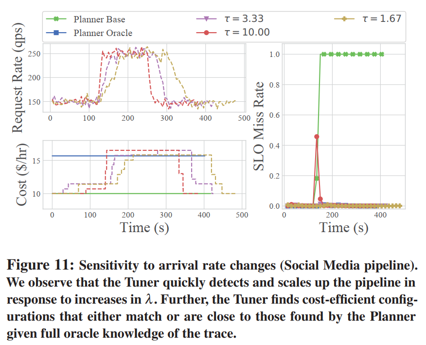
Figures 11 and 12 above show the Tuner’s sensitivity:

1. Planner Oracle knows the entire request sequence at the beginning but has no Tuner, thus consistently using higher cost to avoid SLO miss rate, while Planner Base doesn’t know upcoming requests at the beginning, so SLO miss rate increases sharply when requests increase.
2. $τ$ represents the rate at which requests increase from 150QPS to 250QPS. Clearly, when the request change rate is not high, the Tuner can scale the pipeline well, thus ensuring SLO miss rate remains stable and approaches 0, but when requests surge, SLO miss rate also increases to some extent, but the Tuner quickly adjusts the pipeline.
3. When the request curve oscillates, the Tuner can maintain the pipeline without frequent scaling, thus maintaining a very low SLO miss rate.

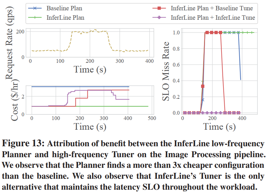
Figure 13 above shows that compared to baseline:

1. InferLine Plan allows the system to have lower initial cost
2. InferLine Tune allows the system to more effectively scale the pipeline when requests increase to ensure SLO targets, and can reduce pipeline replicas when requests decrease, thus allowing the system to have lower cost.

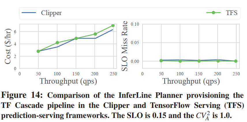
Figure 14 above shows that InferLine achieves the same low latency SLO miss rate for both prediction serving frameworks. This demonstrates the generality of the planning algorithm used to configure individual models in InferLine. The figure shows the SLO achievement rate and pipeline provisioning cost when running InferLine on both serving frameworks. The cost is slightly higher when running on TFS due to some additional RPC serialization overhead not present in Clipper.

Advantages and Disadvantages

Advantages

• InferLine leverages performance profiles for each stage (Profiler) and simulation-based performance estimator (Estimator) to quickly explore the configuration space without running the pipeline.
• Systems like Dhalion and DS2 are throughput-oriented and ignore consideration of sudden traffic arrivals. There are also some systems that consider latency like DRS, Elastic Stream Processing with Latency Guarantees, Nephele Streaming, but they consider average latency. InferLine targets P99 tail latency and considers configuring pipelines for peak loads.
• Compared to existing similar systems, such as [Autoscale][13], InferLine has better tail latency SLO and cost, and supports batching.
• The four algorithms proposed in this paper naturally align with human thinking and intuition, are relatively easy to understand, and achieve good results at the same time.

Disadvantages

• The system does not consider some scenarios in practical applications. In machine learning, latency may be affected by input; in a specific pair of accelerators AB, A may be faster at small batch sizes and slower at large batch sizes.